Fit a multi-armed Qini curve.

Evaluates treatment allocation policies over a range of budget constraints using generalized Qini curves. Given estimated conditional treatment effects, treatment costs, and evaluation scores, maq computes the optimal treatment allocation at each budget level and estimates the corresponding policy value. The optimization exploits the linear multiple-choice knapsack structure of the allocation problem to compute the full solution path efficiently.

maq(
  reward,
  cost,
  DR.scores,
  budget = NULL,
  target.with.covariates = TRUE,
  R = 0,
  paired.inference = TRUE,
  sample.weights = NULL,
  clusters = NULL,
  tie.breaker = NULL,
  num.threads = NULL,
  seed = 42
)

Arguments

reward	A $n \cdot K$ matrix of test set treatment effect estimates $\hat \tau(X_i)$. (Note: the estimated function $\hat \tau(\cdot)$ should be constructed on a held-out training set)
cost	A $n \cdot K$ matrix of test set costs $C(X_i) > 0$, where entry (i, k) measures the cost of assigning the i-th unit the k-th treatment arm. If the costs do not vary by unit, only by arm, this can also be a K-length vector. (Note: these costs need not be denominated on the same scale as the treatment effect estimates).
DR.scores	An $n \cdot K$ matrix of test set evaluation scores used to form an estimate of Q(B). With known treatment propensities $P[W_i\|X_i]$, these scores can be constructed via inverse-propensity weighting, i.e, with entry (i, k) equal to $\frac{\mathbf{1}(W_i=k)Y_i}{P[W_i=k \| X_i]} - \frac{\mathbf{1}(W_i=0)Y_i}{P[W_i=0 \| X_i]}$. In observational settings where $P[W_i\|X_i]$ has to be estimated, then an alternative is to construct these scores via augmented inverse-propensity weighting (AIPW) - yielding a doubly robust estimate of the Qini curve (for details, see the paper).
budget	The maximum spend per unit, $B_{max}$, to fit the Qini curve on. Setting this to NULL (default) computes the solution path up to the maximum spend per unit at which every unit with positive estimated treatment effect (that is, $\hat \tau_k(X_i) > 0$) is treated.
target.with.covariates	If TRUE (Default), then the policy $\pi_B$ takes covariates $X_i$ into account. If FALSE, then the policy only takes the average reward $\bar \tau = E[\hat \tau(X_i)]$ and average costs $\bar C = E[C(X_i)]$ into account when allocating treatment. This can be used to construct a baseline Qini curve to assess the value of treatment targeting based on covariates.
R	Number of bootstrap replicates for computing standard errors. Default is 0 (only point estimates are computed).
paired.inference	Whether to allow for paired tests with other Qini curves fit on the same evaluation data. If TRUE (Default) then the path of bootstrap replicates are stored in order to perform paired comparisons that account for the correlation between curves evaluated on the same data. This takes memory on the order of $O(RnK)$ and requires the comparison objects to be fit with the same seed and R values as well as the same number of samples.
sample.weights	Weights given to an observation in estimation. If NULL, each observation is given the same weight. Default is NULL.
clusters	Vector of integers or factors specifying which cluster each observation corresponds to, which are used to construct clustered standard errors. Default is NULL (ignored).
tie.breaker	An optional permutation of the integers 1 to n used to break potential ties in the optimal treatment allocation (only relevant if the predictions $\hat \tau(X)$ are not continuous). If NULL, the ties are broken by the lowest sample id (i.e. the sample appearing first in the data). Default is NULL.
num.threads	Number of threads used in bootstrap replicates. By default, the number of threads is set to the maximum hardware concurrency.
seed	The seed of the C++ random number generator. Default is 42.

Value

A fit maq object.

Details

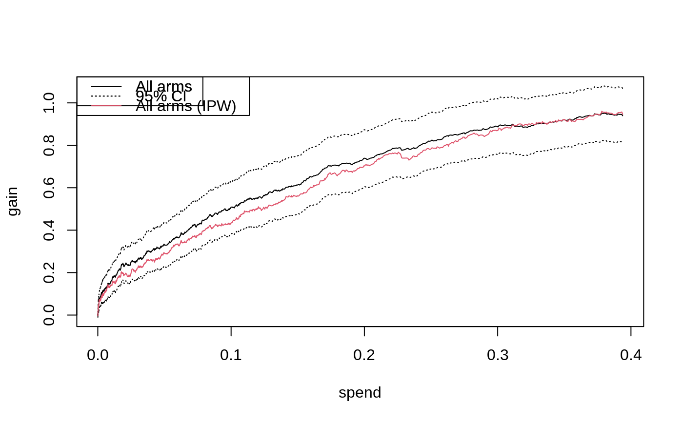
Consider $k = 1, \ldots, K$ mutually exclusive and costly treatment arms, where k = 0 is a zero-cost control arm. Let $\hat \tau(\cdot)$ be an estimated multi-armed treatment effect function and $C(\cdot)$ a known cost function (where the k-th element of these vectors measures $E[Y_i(k) - Y_i(0) | X_i]$ and $E[C_i(k) - C_i(0) | X_i]$ where $Y_i(k)$ are potential outcomes corresponding to the k-th treatment state, $C_i(k)$ the cost of assigning unit i the k-th arm, and $X_i$ a set of covariates). This function provide estimates of the Qini curve: $$Q(B) = E[\langle \pi_B(X_i), \tau(X_i)\rangle], B \in (0, B_{max}],$$ which is the expected gain, at any budget constraint B, when assigning treatment in accordance to $\pi_B$, the treatment policy that optimally selects which arm to assign to which unit while incurring a cost less than or equal to B in expectation when using the given functions $\hat \tau(\cdot)$ and $C(\cdot)$: $$\pi_B = argmax_{\pi} \left\{E[\langle \pi(X_i), \hat \tau(X_i) \rangle]: E[\langle \pi(X_i), C(X_i) \rangle] \leq B \right\}.$$ At a budget B, the k-th element of $\pi_B(X_i)$ is 1 if assigning the k-th arm to the i-th unit is optimal, and 0 otherwise. The Qini curve can be used to quantify the value, as measured by the expected gain over assigning each unit the control arm when using the estimated function $\hat \tau(\cdot)$ with cost structure $C(\cdot)$ to allocate treatment, as we vary the available budget $B$.

References

Sverdrup, Erik, Han Wu, Susan Athey, and Stefan Wager. "Qini Curves for Multi-Armed Treatment Rules". Journal of Computational and Graphical Statistics. 34(3), 2025.

Examples

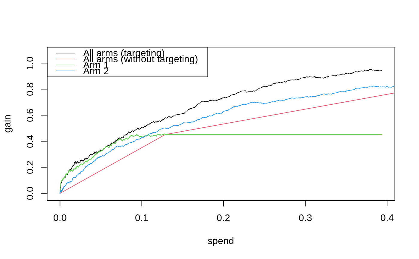
# \donttest{
if (require("grf", quietly = TRUE)) {
# Fit a CATE estimator on a training sample.
n <- 3000
p <- 5
X <- matrix(runif(n * p), n, p)
W <- as.factor(sample(c("0", "1", "2"), n, replace = TRUE))
Y <- X[, 1] + X[, 2] * (W == "1") + 1.5 * X[, 3] * (W == "2") + rnorm(n)
train <- sample(1:n, n/2)

tau.forest <- grf::multi_arm_causal_forest(X[train, ], Y[train], W[train])

# Predict CATEs on held out evaluation data.
test <- -train
tau.hat <- predict(tau.forest, X[test, ], drop = TRUE)$predictions

# Assume costs equal a unit's pre-treatment covariate - the following is a toy example.
cost <- cbind(X[test, 4] / 4, X[test, 5])

# Fit an evaluation forest to compute doubly robust scores on the test set.
eval.forest <- grf::multi_arm_causal_forest(X[test, ], Y[test], W[test])
DR.scores <- grf::get_scores(eval.forest, drop = TRUE)

# Fit a Qini curve on evaluation data, using 200 bootstrap replicates for confidence intervals.
ma.qini <- maq(tau.hat, cost, DR.scores, R = 200)

# Plot the Qini curve.
plot(ma.qini)
legend("topleft", c("All arms", "95% CI"), lty = c(1, 3))

# Get an estimate of gain at a given spend per unit along with standard errors.
average_gain(ma.qini, spend = 0.2)

# Get the treatment allocation matrix at a given spend per unit.
pi.mat <- predict(ma.qini, spend = 0.2)

# If the treatment randomization probabilities are known, then an alternative to
# evaluation via AIPW scores is to use inverse-propensity weighting (IPW).
W.hat <- rep(1/3, 3)
IPW.scores <- get_ipw_scores(Y[test], W[test], W.hat)
mq.ipw <- maq(tau.hat, cost, IPW.scores)

plot(mq.ipw, add = TRUE, col = 2)
legend("topleft", c("All arms", "95% CI", "All arms (IPW)"), col = c(1, 1, 2), lty = c(1, 3, 1))

# Estimate some baseline policies.
# a) A policy that ignores covariates and only takes the average reward/cost into account.
qini.avg <- maq(tau.hat, cost, DR.scores, target.with.covariates = FALSE, R = 200)

# b) A policy that only uses arm 1.
qini.arm1 <- maq(tau.hat[, 1], cost[, 1], DR.scores[, 1], R = 200)

# c) A policy that only uses arm 2.
qini.arm2 <- maq(tau.hat[, 2], cost[, 2], DR.scores[, 2], R = 200)

plot(ma.qini, ci.args = NULL)
plot(qini.avg, col = 2, add = TRUE, ci.args = NULL)
plot(qini.arm1, col = 3, add = TRUE, ci.args = NULL)
plot(qini.arm2, col = 4, add = TRUE, ci.args = NULL)
legend("topleft", c("All arms (targeting)", "All arms (without targeting)", "Arm 1", "Arm 2"),
       col = 1:4, lty = 1)

# Estimate the value of employing all arms over a random allocation.
difference_gain(ma.qini, qini.avg, spend = 0.2)

# Estimate the value of targeting with both arms as opposed to targeting with only arm 1.
difference_gain(ma.qini, qini.arm1, spend = 0.2)

# Estimate the value of targeting with both arms as opposed to targeting with only arm 2.
difference_gain(ma.qini, qini.arm2, spend = 0.2)

# Compare targeting strategies over a range of budget values by estimating an area between
# two curves up to a given spend point.
integrated_difference(ma.qini, qini.arm1, spend = 0.3)
}
#>   estimate    std.err 
#> 0.04856414 0.02722023 
# }

reward	A \(n \cdot K\) matrix of test set treatment effect estimates \(\hat \tau(X_i)\). (Note: the estimated function \(\hat \tau(\cdot)\) should be constructed on a held-out training set)
cost	A \(n \cdot K\) matrix of test set costs \(C(X_i) > 0\), where entry (i, k) measures the cost of assigning the i-th unit the k-th treatment arm. If the costs do not vary by unit, only by arm, this can also be a K-length vector. (Note: these costs need not be denominated on the same scale as the treatment effect estimates).
DR.scores	An \(n \cdot K\) matrix of test set evaluation scores used to form an estimate of Q(B). With known treatment propensities \(P[W_i\|X_i]\), these scores can be constructed via inverse-propensity weighting, i.e, with entry (i, k) equal to \(\frac{\mathbf{1}(W_i=k)Y_i}{P[W_i=k \| X_i]} - \frac{\mathbf{1}(W_i=0)Y_i}{P[W_i=0 \| X_i]}\). In observational settings where \(P[W_i\|X_i]\) has to be estimated, then an alternative is to construct these scores via augmented inverse-propensity weighting (AIPW) - yielding a doubly robust estimate of the Qini curve (for details, see the paper).
budget	The maximum spend per unit, \(B_{max}\), to fit the Qini curve on. Setting this to NULL (default) computes the solution path up to the maximum spend per unit at which every unit with positive estimated treatment effect (that is, \(\hat \tau_k(X_i) > 0\)) is treated.
target.with.covariates	If TRUE (Default), then the policy \(\pi_B\) takes covariates \(X_i\) into account. If FALSE, then the policy only takes the average reward \(\bar \tau = E[\hat \tau(X_i)]\) and average costs \(\bar C = E[C(X_i)]\) into account when allocating treatment. This can be used to construct a baseline Qini curve to assess the value of treatment targeting based on covariates.
R	Number of bootstrap replicates for computing standard errors. Default is 0 (only point estimates are computed).
paired.inference	Whether to allow for paired tests with other Qini curves fit on the same evaluation data. If TRUE (Default) then the path of bootstrap replicates are stored in order to perform paired comparisons that account for the correlation between curves evaluated on the same data. This takes memory on the order of \(O(RnK)\) and requires the comparison objects to be fit with the same seed and R values as well as the same number of samples.
sample.weights	Weights given to an observation in estimation. If NULL, each observation is given the same weight. Default is NULL.
clusters	Vector of integers or factors specifying which cluster each observation corresponds to, which are used to construct clustered standard errors. Default is NULL (ignored).
tie.breaker	An optional permutation of the integers 1 to n used to break potential ties in the optimal treatment allocation (only relevant if the predictions \(\hat \tau(X)\) are not continuous). If NULL, the ties are broken by the lowest sample id (i.e. the sample appearing first in the data). Default is NULL.
num.threads	Number of threads used in bootstrap replicates. By default, the number of threads is set to the maximum hardware concurrency.
seed	The seed of the C++ random number generator. Default is 42.