This document provides a short introduction to the policytree package, with examples from Zhou, Athey and Wager (2023), and Athey and Wager (2021). The last section contains details on the runtime of policy_tree.

library(policytree)
library(grf)

Ex. 1: Binary treatment effect estimation and policy learning

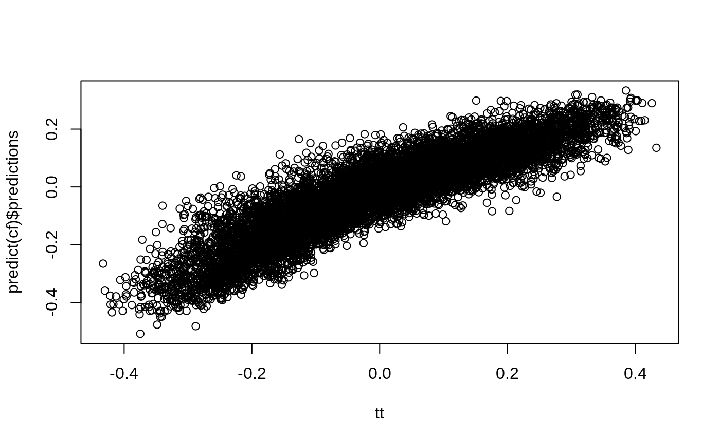
n <- 10000
p <- 10

X <- matrix(rnorm(n * p), n, p)
ee <- 1 / (1 + exp(X[, 3]))
tt <- 1 / (1 + exp((X[, 1] + X[, 2]) / 2)) - 0.5
W <- rbinom(n, 1, ee)
Y <- X[, 3] + W * tt + rnorm(n)

cf <- causal_forest(X, Y, W)

plot(tt, predict(cf)$predictions)

dr <- double_robust_scores(cf)
tree <- policy_tree(X, dr, 2)
tree
#> policy_tree object 
#> Tree depth:  2 
#> Actions:  1: control 2: treated 
#> Variable splits: 
#> (1) split_variable: X2  split_value: -0.287989 
#>   (2) split_variable: X1  split_value: 1.40486 
#>     (4) * action: 2 
#>     (5) * action: 1 
#>   (3) split_variable: X1  split_value: -0.729217 
#>     (6) * action: 2 
#>     (7) * action: 1
pp <- predict(tree, X)
boxplot(tt ~ pp)

plot(tree)

plot(X[, 1], X[, 2], col = pp)
abline(0, -1, lwd = 4, col = 4)

Ex. 2: Multi-action treatment effect estimation

The following example is from the 3-action DGP from section 6.4.1 in Zhou, Athey and Wager

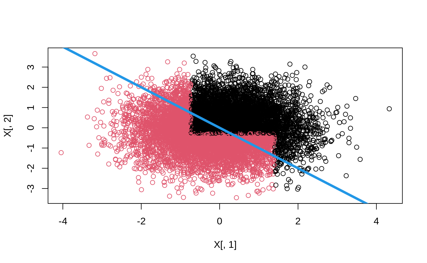
n <- 10000
p <- 10
data <- gen_data_mapl(n, p)
head(data.frame(data)[1:6])
#>   action          Y        X.1       X.2       X.3        X.4
#> 1      1  2.6284326 0.67222112 0.1911761 0.8306201 0.04823820
#> 2      2 -0.4104820 0.06268746 0.5293111 0.9005144 0.17141539
#> 3      0  2.5760171 0.96091759 0.2426804 0.8510604 0.81590389
#> 4      1  6.4251811 0.28812068 0.5097512 0.2848444 0.26683712
#> 5      1 -0.7418237 0.24016147 0.9975204 0.5635440 0.29509120
#> 6      2 -0.1215063 0.12274854 0.8569016 0.4839027 0.09840055

X <- data$X
Y <- data$Y
W <- as.factor(data$action)

multi.forest <- multi_arm_causal_forest(X, Y, W)

# tau.hats:
head(predict(multi.forest)$predictions[,,])
#>           1 - 0      2 - 0
#> [1,] -0.9276891 -2.1225131
#> [2,]  0.1134661 -0.4008315
#> [3,]  1.5934793  2.5233362
#> [4,]  1.2891367  1.7283063
#> [5,] -0.8107706 -1.8774527
#> [6,] -0.8944159 -1.9862733

# Each region with optimal action
region.pp <- data$region + 1
plot(X[, 5], X[, 7], col = region.pp)
leg <- sort(unique(region.pp))
legend("topleft", legend = leg - 1, col = leg, pch = 10)

Policy learning

Cross-fitted Augmented Inverse Propensity Weighted Learning (CAIPWL) with the optimal depth 2 tree

Gamma.matrix <- double_robust_scores(multi.forest)
head(Gamma.matrix)
#>              0         1          2
#> [1,] 3.0736228  2.955238  0.9511097
#> [2,] 2.0894077  2.202874 -7.6580111
#> [3,] 7.9397725  1.641079  2.5709358
#> [4,] 0.3621434 11.463961  2.0904497
#> [5,] 2.9600271 -2.878761  1.0825743
#> [6,] 2.7837680  1.889352 -3.7782404

train <- sample(1:n, 9000)
opt.tree <- policy_tree(X[train, ], Gamma.matrix[train, ], depth = 2)
opt.tree
#> policy_tree object 
#> Tree depth:  2 
#> Actions:  1: 0 2: 1 3: 2 
#> Variable splits: 
#> (1) split_variable: X5  split_value: 0.601445 
#>   (2) split_variable: X7  split_value: 0.35004 
#>     (4) * action: 3 
#>     (5) * action: 1 
#>   (3) split_variable: X7  split_value: 0.713839 
#>     (6) * action: 2 
#>     (7) * action: 3

plot(opt.tree)

Predict treatment on held out data

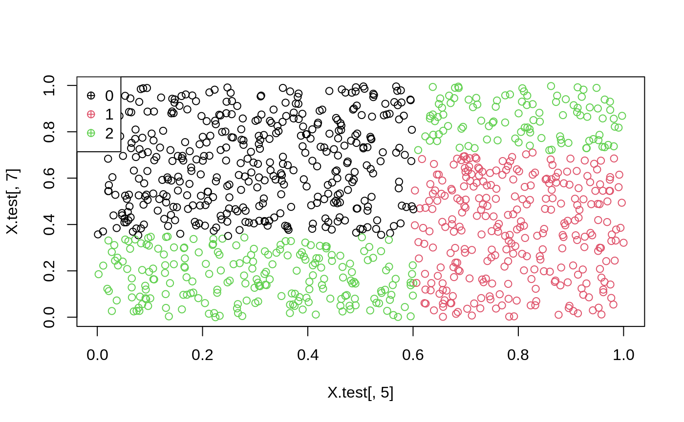
X.test <- X[-train, ]
pp <- predict(opt.tree, X.test)
head(pp)
#> [1] 2 3 1 1 2 2

plot(X.test[, 5], X.test[, 7], col = pp)
leg <- sort(unique(pp))
legend("topleft", legend = leg - 1, col = leg, pch = 10)

Ex. 3: Efficient Policy Learning - Binary Treatment and Instrumental Variables

The following example is from section 5.2 in Wager and Athey (2021).

n <- 500
data <- gen_data_epl(n, type = "continuous")
head(data.frame(data))[1:6]
#>   W Z         tau          Y         X.1         X.2
#> 1 0 1 -0.50000000  3.4662060 -0.13701966 -1.59064506
#> 2 1 1 -0.07788149  0.5532977 -0.84836207  0.84423702
#> 3 0 0  0.17925500  1.4832753  1.02471100  0.33379899
#> 4 0 1 -0.50000000  1.1881457 -0.04921944 -0.85043640
#> 5 1 1  0.09894633  3.1677820  0.32794872  0.86994393
#> 6 0 1 -0.45727715 -0.6397086 -0.79551953  0.08544569

iv.forest <- instrumental_forest(X = data$X, Y = data$Y, W = data$W, Z = data$Z)

gamma <- double_robust_scores(iv.forest)
head(gamma)
#>         control    treated
#> [1,] -2.4074811  2.4074811
#> [2,] -0.9621055  0.9621055
#> [3,]  0.5835709 -0.5835709
#> [4,] -0.7737124  0.7737124
#> [5,] -2.7940823  2.7940823
#> [6,]  4.4812330 -4.4812330

Find the depth-2 tree which solves (2):

train <- sample(1:400)
tree <- policy_tree(data$X[train, ], gamma[train, ])
tree
#> policy_tree object 
#> Tree depth:  2 
#> Actions:  1: control 2: treated 
#> Variable splits: 
#> (1) split_variable: X4  split_value: 0.169516 
#>   (2) split_variable: X1  split_value: 0.503502 
#>     (4) * action: 1 
#>     (5) * action: 2 
#>   (3) split_variable: X1  split_value: -0.389985 
#>     (6) * action: 2 
#>     (7) * action: 1

Evaluate the policy on held out data:

piX <- predict(tree, data$X[-train, ]) - 1
head(piX)
#> [1] 1 1 1 1 1 0

reward.policy <- mean((2 * piX - 1) * data$tau[-train])
reward.policy
#> [1] 0.1524301

Gauging the runtime of tree search

Exact tree search is intended as a way to find shallow (i.e. depth 2 or 3) globally optimal tree-based polices on datasets of “moderate” size. The amortized runtime of the exact tree search is \(O(p^k n^k (log n + d) + pnlog n)\) where \(p\) is the number of features, \(n\) the number of observations, \(d\) the number of treatments, and \(k \geq 1\) the tree depth. Due to the exponents in this expression, exact tree search will not scale to datasets of arbitrary size.

As an example, the runtime of a depth two tree scales quadratically with the number of observations, implying that doubling the number of samples will quadruple the runtime. n refers to the number of distinct observations, substantial speedups can be gained when the features are discrete (with all binary features, the runtime will be ~ linear in n), and it is therefore beneficial to round down/re-encode very dense data to a lower cardinality (the optional parameter split.step emulates this, though rounding/re-encoding allow for finer-grained control).

As a point of reference, the following table presents runtimes for some example problems.

depth	n (continuous)	features	actions	split.step	time
2	1000	30	20	1	1.5 min
2	1000	30	20	10	7 sec
2	10 000	30	20	1	3 hrs
2	10 000	30	20	10	14 min
2	10 000	30	20	1, but `round(X, 2)`	8 min
2	100 000	30	20	10	50 hrs
2	100 000	30	20	1, but `round(X, 2)`	6.3 hrs
2	100 000	60	20	1, but `round(X, 2)`	25 hrs
2	100 000	30	3	10	7.4 hrs

Fitting deeper trees with hybrid search

The previous section demonstrates that it is infeasible to grow globally optimal deep (depth >= 3) trees on very large N. Notice however that with appropriate discretization of continuous covariates, and feature selection, growing depth 2 exact trees is feasible.

We can maintain the depth-2 amortized runtime while growing deeper trees by using a “hybrid” approach: look ahead depth-2 subtrees when forming splits. This heuristic combines the advantages of a fully greedy and fully optimal approach: by looking further ahead we take potential interactions among variables into account, while retaining feasible scaling. This feature is available in hybrid_policy_tree.

An exact depth 3 tree using the dataset above would take almost 10 minutes to complete, compared with the hybrid approach: