Developing

In addition to providing out-of-the-box forests for quantile regression and instrumental variables, grf provides a framework for creating forests tailored to new statistical tasks. Certain components around splitting and prediction can be swapped out, within the general infrastructure for growing and predicting on trees.

Table of Contents

• Contributing
• Working with the code
• R package
  • Note for Windows users
• Core C++
  • Code structure
  • Creating a custom forest
  • Current forests and main components
  • Tree splitting algorithm
  • Computing point predictions

Contributing

This repository follows the standard open source protocol and setup with git where there is an abundance of existing resources to get up to speed (see for example the contributing guidelines for well known packages in other languages, like Scikit-learn, Scipy, and pandas)

Condensed greatly, the workflow is to fork this repository, check out a branch, commit your changes (forming an ideally legible commit history), then submitting a pull request explaining your contribution, ideally referring to the issue you created, or the issue you chose to work on.

Working with the code

The core forest implementation is written in C++, with an R interface powered by Rcpp. We recommend using a full-powered C++ IDE such as CLion, Xcode, or Visual Studio when working with the core code.

R package

To build the R package from source, cd into r-package and run build_package.R. Required development dependencies are listed there. This mimics the tests run when submitting a pull request. Additional online package documentation is built using continuous integration with pkgdown. Usage examples in the form of R Markdown files under grf\vignettes are built and rendered and the R method reference (along with the package articles) is displayed according to the layout defined in pkgdown.yml. To build the site locally run pkgdown::build_site() from the R package directory.

An alternative development workflow is to use the accompanying grf.Rproj and build and test the package with RStudio’s build menu, which can be convenient for quickly iterating C++/R code changes. Compiling the package locally with PKG_CPPFLAGS="-UNDEBUG" (or set in ~/.R/Makevars) may give helpful debug assertions, as the Eigen library will then perform bounds checks on matrix algebra.

Note for Windows users:

Symlinks in the src directory point to the core C++ and R bindings. On Windows one has to clone this repository with symlinks enabled: git clone -c core.symlinks=true https://github.com/grf-labs/grf.git (this command may have to be run as an administrator if the account does not have permission to create symlinks). Caveat: the above RStudio workflow is not tested on Windows.

Core C++

Code structure

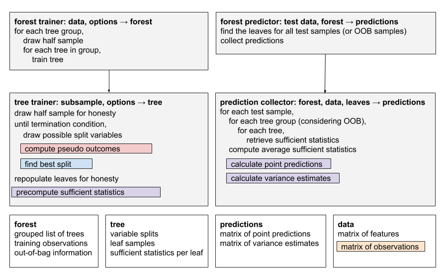
The forest implementation is composed of two top-level components, ForestTrainer and ForestPredictor.

ForestTrainer drives the tree-growing process, and has two pluggable components.

• RelabelingStrategy is applied before every split, and produces a set of relabelled outcomes given the observations for a group of samples. In the case of quantile forests, for example, this strategy computes the quantiles for the group of samples, then relabels them with a factor corresponding to the quantile they belong to.
• SplittingRule is called to find the best split for a particular node, given a set of outcomes. There are currently implementations for standard regression and multinomial splitting.

The trained forest produces a Forest object. This can then be passed to the ForestPredictor to predict on test samples. The predictor has a pluggable ‘prediction strategy’, which computes a prediction given a test sample. Prediction strategies can be one of two types:

• DefaultPredictionStrategy computes a prediction given a weighted list of training sample IDs that share a leaf with the test sample. Taking quantile forests as an example, this strategy would compute the quantiles of the weighted leaf samples.
• OptimizedPredictionStrategy does not predict using a list of neighboring samples and weights, but instead precomputes summary values for each leaf during training, and uses these during prediction. This type of strategy will also be passed to ForestTrainer, so it can define how the summary values are computed. The section on computing point predictions provides more details.

Prediction strategies can also compute variance estimates for the predictions, given a forest trained with grouped trees. Because of performance constraints, only ‘optimized’ prediction strategies can provide variance estimates.

A particular type of forest is created by pulling together a set of pluggable components. As an example, a quantile forest is composed of a QuantileRelabelingStrategy, ProbabilitySplittingRule, and QuantilePredictionStrategy. The factory classes ForestTrainers and ForestPredictors define the common types of forests like regression, quantile, and causal forests.

Creating a custom forest

When designing a forest for a new statistical task, we suggest following the format suggested in the paper: provide a custom RelabelingStrategy and PredictionStrategy, but use the standard RegressionSplittingRule. If modifications to the splitting rule must be made, they should be done carefully, as it is an extremely performance-sensitive piece of code.

To get started with setting up new classes and Rcpp bindings, we suggest having a look at one of the simpler forests, like regression_forest, and use this as a template.

Current forests and main components

The following table shows the current collection of forests implemented and the C++ components.

R forest name	RelabelingStrategy	SplittingStrategy	PredictionStrategy
causal_forest	InstrumentalRelabelingStrategy	InstrumentalSplittingRule	InstrumentalPredictionStrategy
causal_forest with ll_causal_predict	InstrumentalRelabelingStrategy	InstrumentalSplittingRule	LLCausalPredictionStrategy
causal_survival_forest	CausalSurvivalRelabelingStrategy	CausalSurvivalSplittingRule	CausalSurvivalPredictionStrategy
instrumental_forest	InstrumentalRelabelingStrategy	InstrumentalSplittingRule	InstrumentalPredictionStrategy
ll_regression_forest	LLRegressionRelabelingStrategy	RegressionSplittingRule	LocalLinearPredictionStrategy
lm_forest	MultiCausalRelabelingStrategy	MultiRegressionSplittingRule	MultiCausalPredictionStrategy
multi_arm_causal_forest	MultiCausalRelabelingStrategy	MultiCausalSplittingRule	MultiCausalPredictionStrategy
multi_regression_forest	MultiNoopRelabelingStrategy	MultiRegressionSplittingRule	MultiRegressionPredictionStrategy
probability_forest	NoopRelabelingStrategy	ProbabilitySplittingRule	ProbabilityPredictionStrategy
quantile_forest	QuantileRelabelingStrategy	ProbabilitySplittingRule	QuantilePredictionStrategy
regression_forest	NoopRelabelingStrategy	RegressionSplittingRule	RegressionPredictionStrategy
survival_forest	NoopRelabelingStrategy	SurvivalSplittingRule	SurvivalPredictionStrategy

Tree splitting algorithm

The follow section outlines pseudocode for some of the components listed above.

Each splitting rule follow the same pattern: given a set of samples, and a possible split variable, iterate over all the split points for that variable and compute an error criterion on both sides of the split, then select the split where the decrease in the summed error criterion is smallest. For RegressionSplittingRule the criterion is the mean squared error, and is usually referred to as standard CART splitting. InstrumentalSplittingRule use the same error criterion, but it incorporates more constraints on potential splits, such as requiring a certain number of treated and control observations (more details are in the Algorithm Reference).

Two added features to grf’s splitting rule beyond basic CART is the addition of sample weights and support for missing values with Missingness Incorporated in Attributes (MIA) splitting. The algebra behind the decrease calculation is detailed below.

Algorithm (RegressionSplittingRule): find the best split for variable var at n samples samples = i...j

Input: X: covariate matrix, weights: weight n-vector, response: the responses (pseudo-outcomes) n-vector, min_child_size: split constraint on number of samples

Output: The best split value and the direction to send missing values

let x = X[samples, var]

for each unique value u in x:
  let count_left[u] be the number of samples with x <= u
  let sum_left[u], weight_sum_left[u] be the sum of weight * response and weight with x <= u

  let count_right[u], sum_right[u], weight_sum_right[u] be the same for samples with x > u
  let count_missing, sum_missing, weight_sum_missing be the same for samples with x = missing

  decrease[u, missing = on_left] = (sum_left[u] + sum_missing)^2 / (weight_sum_left[u] + weight_sum_missing)
                                  + sum_right[u]^2 / weight_sums_right[u]

  decrease[u, missing = on_right] = sum_left[u]^2 / weight_sum_left[u]
                                  + (sum_right[u] + sum_missing)^2 / (weight_sums_right[u] + weight_sum_missing)

return (u, missing) that maximizes decrease such that
count_left[u] and count_right[u] >= min_child_size

---

Algorithm (Decrease calculation in weighted CART): find the best split Sj for variable Xj. The impurity criterion is the sum of weighted mean squared errors, which for a specific split Sj is minimized by the weighted sample average Ybar (see for example Elements of Statistical Learning, Ch 9).

Input: Xj : Covariate j, w: sample weight vector, y: response vector

Output: The best split criterion

minimize wrt. s: MSE(s, left) + MSE(s, right)

where

MSE(s, left) = \sum_{i \in L(s)} wi [yi - Ybar_L(s)]^2
MSE[s, right] = \sum_{i \in R(s)} wi [yi - Ybar_R(s)]^2

L(s) are all points Xj such that Xj <= s, and R(s) are all points such that Xj > s.
Ybar_L(s) and Ybar_R(s) are the weighted sample averages for the respective partitions.

Expand the child impurity and write out the averages (minimize wrt. s):
= \sum_{i \in L(s)} wi yi^2 - W_L(s) [Ybar_L(s)]^2
 + \sum_{i \in R(s)} wi yi^2 - W_R(s) [Ybar_R(s)]^2
= \sum_i wi yi^2
  - 1/W_L(s) [\sum_{i \in L(s)} wi yi]^2
  - 1/W_R(s) [\sum_{i \in R(s)} wi yi]^2

Where W is the sum of sample weights.

The parent impurity is (minimize wrt. s):
= \sum_i wi [yi - Ybar]^2
= \sum_i wi yi^2 - W Ybar^2
= \sum_i wi yi^2 - 1/W [\sum_i wi yi]^2

Child impurity <= parent impurity then reduces to

1/W_L(s) [\sum_{i \in L(s)} wi yi]^2 + 1/W_R(s) [\sum_{i \in R(s)} wi yi]^2 >= 1/W [\sum_i wi yi]^2

Or sum_left^2 / weight_sum_left + sum_right^2 / weight_sum_right

For multivariate CART sum_left^2 and sum_right^2 becomes the squared L2 norm.

---

Algorithm (SurvivalSplittingRule): find the best split for variable var at n samples samples = i...j.

Input: X: covariate matrix, response: the failure times, min_child_size: split constraint on number of failures, m: the number of failure times in this node.

Output: The best split value and the direction to send missing values

grf performs survival splits by finding the partition that maximizes the log-rank test for the comparison of the survival distribution in the left and right node. The statistic is:

logrank(x, split.value) =  sum over all times k up to m
  (dk,l - Yk,l * dk/Yk)  /
  (Yk,l / Yk * (1 - Yk,l / Yk) * (Yk - dk) / (Yk - 1) dk)

dk,l: the count of failures in the left node at time k
Yk,l: the count of observations at risk in the left node at time k (At risk: all i such that Ti >= k)
dk: the count of failures in the parent node at time k
Yk: the count of observations at risk in the parent node at time k

Note that the absolute value of the response variable (the failure time) is never used, only counts matter, constructed from the relative ordering between them. Therefore, the response variable is always relabeled to range from consecutive integers starting at zero and ending at the number of failures. This can be done quickly with binary search:

let failure_times be a sorted vector of the original failure values (T1, T2, .. TM)
initialize response_relabeled = zeros(n)
for each i=1:n
  relabeled_failure_time = binary_search(response[i], failure_times)
  response_relabeled[i] = relabeled_failure_time

A label of 0 is given to all samples with response less than the first failure time, a value of 1 is given to all samples with failure value greater or equal to the first failure value and less than the second failure value, etc.

The algorithm proceeds in the same manner as outlined above for RegressionSplitting: iterate over all possible splits and calculate the logrank statistic, one with all missing values on the left, and one with all missing on the right. Then select the split that yielded the maximum logrank test, subject to a constraint that there are a sufficient amount of failures on both sides of the split.

---

Algorithm (ProbabilitySplittingRule): This splitting rule uses the Gini impurity measure from CART for categorical data. Sample weights are incorporated by counting the sample weight of an observation when forming class counts. The missing values adjustment is the same as for the other splitting rules.

Computing point predictions

GRF point estimates, θ(x), for a target sample X = x, are given by a forest-specific estimating equation ψ_θ(x)( ⋅ ) solved using GRF forest weights α(x) (see equation (2) and (3) in the GRF paper). In the GRF software package we additionally incorporate sample weights w_i. For training samples i = 1...n, predictions at a target sample X = x are given by:

$$ \sum_{i = 1}^{n} \alpha_i(x) w_i \psi_{\theta(x)}(\cdot) = 0. $$

This is the construction the DefaultPredictionStrategy operates with. The forest weights α_i(x) are available through the method parameter weights_by_sample: entry i is the fraction of times the i-th training sample falls into the same leaf as the target sample x.

For performance reasons, this is not the construction used for most forest predictions, since for many statistical tasks doing this summation over n training samples times the number of target samples involves redundant (repeated) computations. The OptimizedPredictionStrategy avoids this drawback by relying on precomputed forest-specific ‘sufficient’ statistics.

Example: regression forest

We’ll illustrate with an example for regression forest. The estimating equation for the conditional mean μ(x) is ψ_μ(x)(Y_i) = Y_i − μ(x). Plugging this into the moment equation above gives:

$$ \sum_{i = 1}^{n} \alpha_i(x) w_i (Y_i - \mu(x)) = 0. $$

Solving for μ(x) gives

$$ \mu(x) = \frac{\sum_{i = 1}^{n} \alpha_i(x) w_i Y_i}{\sum_{i = 1}^{n} \alpha_i(x) w_i}. $$

Now, insert the definition of the forest weights:

$$ \alpha_i(x) = \frac{1}{B}\sum_{b=1}^{B} \frac{I(X_i\in L_b(x) )}{|L_b(x)|}, $$

where L_b(x) is the set of training samples falling into the same leaf as x in the b-th tree and |L_b(x)| is the cardinality of this set. This gives us:

$$ \mu(x) = \frac{\sum_{i = 1}^{n} \bigg(\frac{1}{B}\sum_{b=1}^{B} \frac{I(X_i\in L_b(x) )}{|L_b(x)|}\bigg) w_i Y_i}{\sum_{i = 1}^{n} \bigg(\frac{1}{B}\sum_{b=1}^B \frac{I(X_i\in L_b(x) )}{|L_b(x)|}\bigg) w_i}. $$

Now we change the order of summation, moving the summation over trees outside:

$$ \begin{split} \mu(x) &= \frac{\frac{1}{B} \sum_{b = 1}^{B} \bigg( \frac{1}{|L_b(x)|}\sum_{i=1}^{n} I(X_i\in L_b(x) ) w_i Y_i\bigg)}{\frac{1}{B} \sum_{b = 1}^{B} \bigg(\frac{1}{|L_b(x)|}\sum_{i=1}^{n} I(X_i\in L_b(x) ) w_i\bigg)} \\ &= \frac{\frac{1}{B} \sum_{b = 1}^{B} \bar Y_b(x)} {\frac{1}{B} \sum_{b = 1}^{B} \bar w_b(x)}, \end{split} $$

where we define the two tree-specific sufficient statistics Ȳ_b(x) and w̄_b(x) as:

$$ \bar Y_b(x) =\frac{1}{|L_b(x)|}\sum_{i=1}^{n} I(X_i\in L_b(x) ) w_i Y_i, $$

and

$$ \bar w_b(x) =\frac{1}{|L_b(x)|}\sum_{i=1}^{n} I(X_i\in L_b(x) ) w_i. $$

That is, computing a point estimate for μ(x) now involves a summation of B pre-computed sufficient statistic (done during training in the method precompute_prediction_values).

Example: causal forest

Causal forest and instrumental forest shares the same implementation since a causal forest equals an instrumental forest with the treatment assignment vector equal to the instrument. For simplicity, we here just state what the above decomposition would look like for a causal forest (see section 6.1 of the GRF paper), given centered outcomes and treatment assignments (Ỹ_i, W̃_i) (see section 6.1.1 of the GRF paper). The point predictions τ(x) for target sample X = x are given by:

$$ \tau(x) = \frac{\frac{1}{B} \sum_{b = 1}^{B} \bigg( \bar {YW}_b(x) \bar w_b(x) - \bar Y_b(x) \bar W_b(x) \bigg)} {\frac{1}{B} \sum_{b = 1}^{B} \bigg( \bar W^2_b(x) \bar w_b(x) - \bar W_b(x) \bar W_b(x) \bigg) }, $$

where

$$ \bar Y_b(x) = \frac{1}{|L_b(x)|}\sum_{i=1}^{n} I(X_i\in L_b(x) ) w_i \tilde Y_i, $$

$$ \bar W_b(x) = \frac{1}{|L_b(x)|}\sum_{i=1}^{n} I(X_i\in L_b(x) ) w_i \tilde W_i, $$

$$ \bar W^2_b(x) = \frac{1}{|L_b(x)|}\sum_{i=1}^{n} I(X_i\in L_b(x) ) w_i \tilde W^2_i, $$

$$ \bar w_b(x) =\frac{1}{|L_b(x)|}\sum_{i=1}^{n} I(X_i\in L_b(x) ) w_i, $$

$$ \bar {YW}_b(x) =\frac{1}{|L_b(x)|}\sum_{i=1}^{n} I(X_i\in L_b(x) ) w_i \tilde Y_i \tilde W_i. $$