library(grf)
This vignette gives a brief beginner-friendly overview of how
non-parametric estimators like GRF can be used to flexibly estimate
treatment effects in a survival setting where we want to remain agnostic
on assumptions for the censoring and survival process. The first part of
this vignette gives a basic intro to right-censored data and issues with
estimating an average survival time. The second part shows how GRF can
use sample.weights to construct an IPCW-based causal_forest,
and explains the more powerful estimation approach available in the
function causal_survival_forest.
Right-censored data
 Imagine we are interested in estimating \(E[T]\): how long on average it takes before
a sea otter pup catches its first prey. We drive down to Moss Landing
approximately one hour away from Stanford campus and equip a handful of
same-age pups with a device which tells us if it catches a sea urchin,
scallop, crab, etc. Due to limited funds and time constraints our study
ends after 10 days. During these 10 days our measurement device may also
fail randomly (batteries may stop working - they run out completely
after 12 days, it malfunctions, etc.). This means that for some of our
subjects instead of observing the time they catch a prey we observe when
the device stops working, i.e. the time at which they get censored:
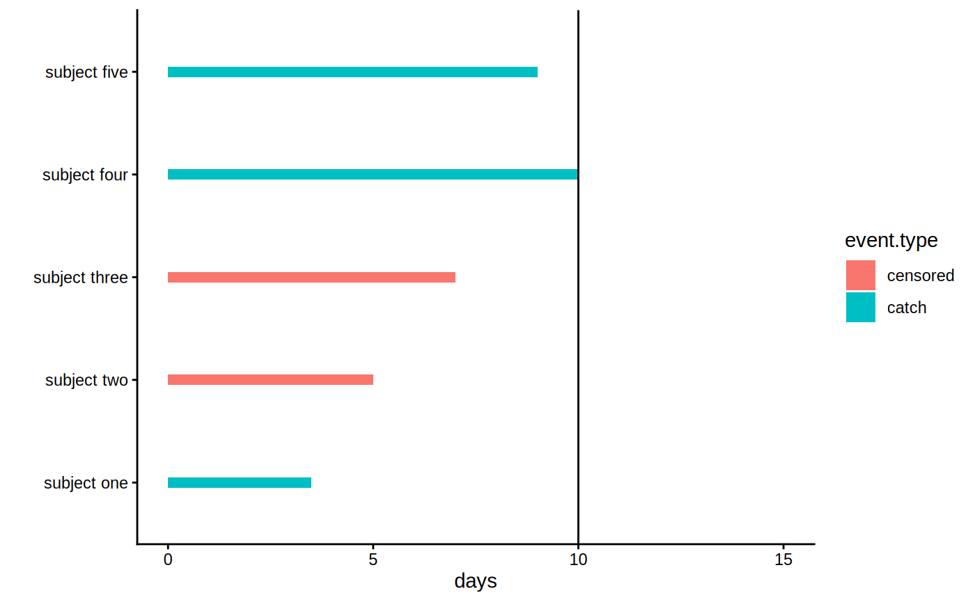
\(C\). The following graph illustrates
what this data may look like, the black bar denotes the study end.
Imagine we are interested in estimating \(E[T]\): how long on average it takes before
a sea otter pup catches its first prey. We drive down to Moss Landing
approximately one hour away from Stanford campus and equip a handful of
same-age pups with a device which tells us if it catches a sea urchin,
scallop, crab, etc. Due to limited funds and time constraints our study
ends after 10 days. During these 10 days our measurement device may also
fail randomly (batteries may stop working - they run out completely
after 12 days, it malfunctions, etc.). This means that for some of our
subjects instead of observing the time they catch a prey we observe when
the device stops working, i.e. the time at which they get censored:
\(C\). The following graph illustrates
what this data may look like, the black bar denotes the study end.
Right-censored data
Subject two and three: their measurement device malfunctions and they drop out of the study, all we know is they had not caught anything at the last measurement time. Subjects one, four, and five catch their first prey during the first 10 days.
This setup describes a typical data collection process in time-to-event studies called right-censoring. Instead of observing a subject’s event time \(T_i\) we observe \(Y_i\) defined as
\[\begin{equation} Y_i = \begin{cases} T_i & \text{if} \, T_i \leq C_i \\ C_i & \text{otherwise} \end{cases} \end{equation}\]
along with an event indicator \(D_i\)
\[\begin{equation} D_i = \begin{cases} 1 & \text{if} \, T_i \leq C_i \\ 0 & \text{otherwise.} \end{cases} \end{equation}\]
In our example subject one, four and five all experienced the event (\(D=1\)) while two and three did not (\(C=0\)). Since in survival settings the event taking place is often a death, the event times \(T\) are often referred to as failure times.
We’ll proceed by making matters concrete with a simulated toy example. Let the time until a pup gets its first catch follow an exponential distribution with rate \(0.1\) i.e. \(T \sim \textrm{Exp}(0.1)\). Let the measurement device be equally likely to malfunction any time during the lifespan of the device, i.e the censoring probability is uniformly distributed with \(C \sim U(0, 12)\). If we plot the distribution of observed events \(D\cdot T\) as well as the distribution of \(T\) they would look like:
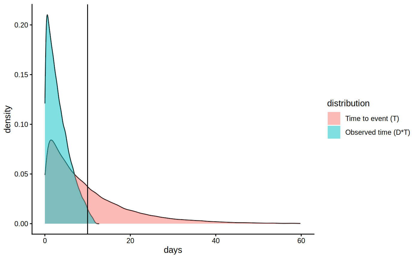
Densities
One immediate thing to note from this plot is that we have to revise our target estimand: it is actually not possible to estimate the mean of \(T\) as its density has support all the way up to 60+ days, and our study ends at 10 days. What we can estimate is a truncated mean, which we call the restricted mean survival time (RMST) defined as
\[E[\min(T, h)] = E[T \land h],\]
where \(h\) is a truncation parameter
(called horizon in the GRF package). If we set \(h=10\) we can see from the plot that \(E[T \land h]\) is defined since we observe
events (blue graph) all up until \(t=10\) days. Let’s denote our new truncated
survival time by \(\hat T = T \land
h\). This truncation also implies an updated event indicator: all
samples still tracked at time \(h\) are
considered as having an observed event at time \(h\) regardless whether they are censored or
not because we know they must not have experienced the event at time
\(h\). Denote this by \(\hat D = \max(D, \, 1\{T\geq h\})\). This
looks like:
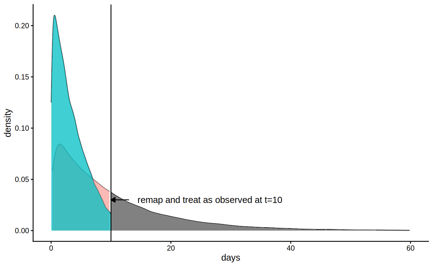
Truncated densities
From this plot it is evident that we can’t estimate \(E[\hat T]\) using only the observed events, we need to take censoring into account, otterwise we’ll get biased estimates. As seen from the plots, the two densities overlap, with significant mass in all regions up to \(h\), which means that if we know the censoring probabilities, we can use inverse probability weighting to upweight the observed events and recover an unbiased estimate of \(E[\hat T]\). Define the censoring probabilities \(P[C > \hat T \,|\, \hat T] = E[\hat D \,|\, \hat T]\). If we upweight the observed events by \(1 / E[\hat D \,|\, \hat T]\) we get (using the law of iterated expectations):
\[\begin{equation*} \begin{split} & E\left[\frac{\hat D \hat T}{E[\hat D \,|\, \hat T]}\right] \\ &= E\left[ E\left[\frac{\hat D \hat T}{E[\hat D \,|\, \hat T]} \,\big|\, \hat T \right]\right] \\ &= E\left[\frac{\hat T}{E[\hat D \,|\, \hat T]} E[\hat D \,|\, \hat T]\right] \\ &= E[\hat T]. \end{split} \end{equation*}\]
The following code snippet illustrates with a toy example:
n <- 100000
event.time <- rexp(n, rate = 0.1)
censor.time <- runif(n, 0, 12)
Y <- pmin(event.time, censor.time)
D <- as.integer(event.time <= censor.time)

# Define the new truncated Y and updated event indicator
horizon <- 10
Dh <- pmax(D, Y >= horizon)
Yh <- pmin(Y, horizon)

observed.events <- (Dh == 1)
censoring.prob <- 1 - punif(Yh[observed.events], 0, 12) # P(C > T)
sample.weights <- 1 / censoring.prob

mean(pmin(event.time, horizon)) # True unobserved truncated mean
#> [1] 6.33776
mean(Yh[observed.events]) # Biased
#> [1] 4.076917
weighted.mean(Yh[observed.events], sample.weights) # IPC weighted
#> [1] 6.367093
This section suggests one way to adopt a causal_forest
for right-censored data would be inverse probability of censoring
weighting (IPCW) and an important purely mechanical observation can
be made before the subsequent CATE estimation paragraph: to get stable
estimates we would like for \(P[C_i >
T_i]\) to not get too low as that implies explosive sample
weights. Intuitively from the density plot, we want to set a threshold
that has “considerable” probability of still observing events, if the
tail is very thin our estimation task is harder.
CATE estimation and right-censored data
Continuing with the fictional experimental setup described in the beginning, imagine instead we randomly split the otter pups into two groups: treated (\(W=1\)) and control (\(W=0\)). The treated group is given hunting lessons that we think helps them catch prey more effectively. The control group is given nothing. We also gather some subject specific covariates \(X\) like \(X_1\)=otter size, etc. We are interested in measuring the expected difference in outcomes (RMST) conditional on covariates, defined as:
\[\tau(x) = E[T(1) \land h - T(0) \land h \, | X = x],\] where \(T(1)\) and \(T(0)\) are potential outcomes corresponding to the two treatment states. In order to estimate this we require something beyond the standard identifying assumptions for CATE estimation with observational data (unconfoundedness/ignorability and overlap).
As the example in the previous section made clear, the censoring mechanism was completely random (failing batteries and measuring devices). This is a crucial assumption, and we require:
- Ignorable censoring: censoring is independent of survival time conditionally on treatment and covariates, \(T_i \perp C_i \mid X_i, \, W_i\).
We can get a sense of what the second identifying assumption is by
looking at the density plots from the previous section. We saw that for
the restricted mean to be identified, we needed there to be some chance
of observing an event during our study period, captured by the
horizon parameter \(h\).
This second assumption make that requirement:
- Positivity: each subject has some probability of having an event observed, \(P[C_i < h \, | X_i, \, W_i] \leq 1 - \eta_C\) for some \(\eta_C > 0\).
Continuing with the simple stylized example from the first section, we simulate the following setup, where we stop collecting samples after t=10 days, with random treatment assignment and where \(\tau(X)\) depends on the first covariate \(X_1\).
n <- 700
p <- 5
X <- matrix(runif(n * p), n, p)
colnames(X) <- c("size", "fur.density", "x3", "x4", "x5")
W <- rbinom(n, 1, 0.5)
horizon <- 10
event.time <- pmin(rexp(n, rate = 0.1 + W * X[, 1]), horizon)
censor.time <- runif(n, 0, 12)
Y <- round(pmin(event.time, censor.time), 1)
D <- as.integer(event.time <= censor.time)
Causal forest with sample weights
This section shows how we can use estimated sample weights to adopt
causal_forest for IPCW estimation. Most GRF estimators have
an optional sample.weights argument which is taken into
account during all steps of the GRF algorithm
(relabeling/splitting/prediction). We start by using a survival_forest
to estimate the censoring process \(P[C_i >
t \, | X_i = x, W_i = w]\), then pick out the appropriate
censoring probabilities \(P[C_i > \hat T_i
\, | X_i = x, W_i = w]\). In our example the censoring
probabilities are “easy” to estimate: they are all uniform. However,
many applications involve more complex censoring patterns, it would not
be unreasonable to expect that the size of the otter pup mattered for
the censoring probabilities, as a larger pup might allow the measurement
device to be strapped on more securely and thus less likely to break
than on a smaller pup. Estimating \(P[C_i >
t \, | X_i = x, W_i = w]\) non-parametrically with GRF’s
survival_forest allows us to be agnostic to this.
sf.censor <- survival_forest(cbind(X, W), Y, 1 - D)
sf.pred <- predict(sf.censor, failure.times = Y, prediction.times = "time")

censoring.prob <- sf.pred$predictions
observed.events <- (D == 1)
sample.weights <- 1 / censoring.prob[observed.events]
Note: when doing inverse weighting it is usually a good idea to plot
the histogram of the weights to get a sense of stability behavior. If
you look at the simulated data, we also discretize the event values by
rounding: this is done because training a survival forest involves
estimating a survival curve on a grid consisting of all unique event
times, and having this grid unreasonably dense brings little benefits
w.r.t statistical accuracy over the extra computational cost (the
optional failure.times argument embeds this
functionality).
Putting everything together we train a causal forest on all observed
events, and pass in the appropriate sample weights. Since we know our
study is randomized with equal treatment assignment we also supply the
know propensity score W.hat \(=E[W_i \, | X_i = x] = 0.5\):
cf <- causal_forest(X[observed.events, ], Y[observed.events], W[observed.events],
                    W.hat = 0.5, sample.weights = sample.weights)

average_treatment_effect(cf)
#>  estimate   std.err
#> -4.745934  0.491739
The ATE is negative, which suggests that hunting lessons make the otter pup catch their first prey in fewer days than those in the control group. That is, the treatment has a positive estimated impact.
Causal survival forest (CSF)
Two drawbacks with the previous approach are:
- It relies on estimated censoring probabilities, and IPCW type estimators are typically not robust to estimation errors in these.
- It only considers observations with observed events. If many subjects are censored this suggests an efficiency loss.
The method implemented in the function
causal_survival_forest alleviates these drawbacks by
leveraging insights from the survival literature on censoring robust
estimating equations (Robins et al., 1994, Tsiatis, 2007). It does so by
taking the (complete-data) causal forest estimating equation \(\psi^{(c)}_{\tau(x)}(T, W, ...)\) (the
“R-learner”) and turn it into a censoring robust estimating equation
\(\psi_{\tau(x)}(Y, W, ...)\) by using
estimates of the survival and censoring processes \(P[C_i > t \, | X_i = x, W_i = w], \, P[T_i >
t \, | X_i = x, W_i = w]\) (“\(...\)” refers to additional nuisance
parameters). The upshot of this “orthogonal” estimating equation is that
it will be consistent if either the survival or censoring process is
correctly specified, which is very beneficial when we want to estimate
these by modern ML tools, such as random survival forests. For more
details see the causal survival forest paper.
We estimate this by specifying target = "RMST" and
supplying the given horizon of t=10 days:
csf <- causal_survival_forest(X, Y, W, D, W.hat = 0.5, target = "RMST", horizon = 10)

average_treatment_effect(csf)
#>   estimate    std.err
#> -4.3136116  0.2486059
The associated standard errors are smaller than in the previous section since unlike causal forest, CSF does not only use observations with observed events. (Note: when running the command you may see a warning that some estimated censoring probabilities are less than 0.2, this is fine for this application, CSF is just being conservative since as noted previously our estimation approach involves division by these).
We can use best_linear_projection to estimate a linear
effect modification measure, and can see that an otter’s size has
significant impact, hunting lessons have a greater effect for bigger
otter pups:
best_linear_projection(csf, X)
#>
#> Best linear projection of the conditional average treatment effect.
#> Confidence intervals are cluster- and heteroskedasticity-robust (HC3):
#>
#>             Estimate Std. Error t value Pr(>|t|)
#> (Intercept) -0.51799    1.00054 -0.5177  0.60482
#> size        -4.31787    0.90276 -4.7830 2.11e-06 ***
#> fur.density -1.64467    0.85832 -1.9162  0.05576 .
#> x3          -0.92173    0.83811 -1.0998  0.27181
#> x4          -0.73406    0.88210 -0.8322  0.40560
#> x5          -0.16570    0.83810 -0.1977  0.84333
#> ---
#> Signif. codes:  0 '***' 0.001 '**' 0.01 '*' 0.05 '.' 0.1 ' ' 1
We can plot the TOC curve by otter weight to assess how heterogeneity varies by a given covariate.
rate <- rank_average_treatment_effect(csf, X[, "size"])
plot(rate, ylab = "Days until first catch", main = "TOC: ranked by decreasing weight")
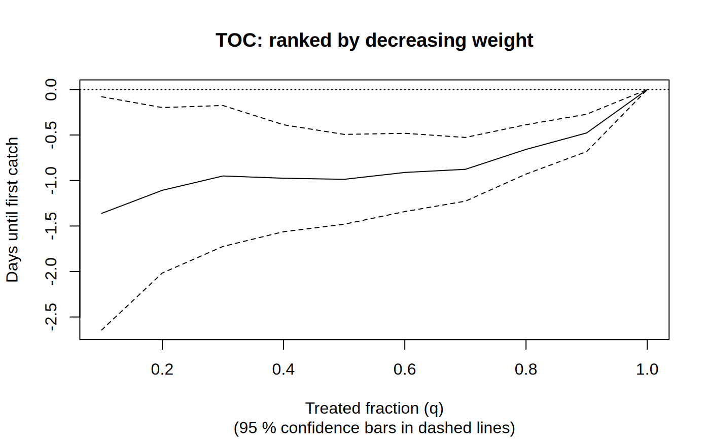
# Estimate of the area under the TOC
rate
#>    estimate   std.err             target
#>  -0.9667595 0.2476909 priorities | AUTOC
Other estimation targets: survival probabilities
CSF can also be used to estimate the difference in survival
probabilities. This option is available through the argument
target = "survival.probability" and estimates for a given
horizon \(h\):
\[\tau(x) = P[T(1) > h \, | X = x] - P[T(0) > h \, | X = x].\]
This extension can be made using the estimation framework described in the previous section. The rest of this vignette contains details on the general setup. Let \(y(\cdot)\) be a deterministic function that satisfies the following:
- Finite horizon: The outcome transformation \(y(\cdot)\) admits a maximal horizon \(0 < h < \infty\), such that \(y(t) = y(h)\) for all \(t \geq h\).
The CATE can then be defined as \(\tau(x) = E[y(T(1)) - y(T(0)) \, | X = x]\). The restricted mean survival time is given by the outcome transformation \(y(T) = T \land h\), and the survival function is given by the outcome transformation \(y(T) = 1\{T > h\}\). As noted earlier this setup implies we only need to take into account events occurring up until time \(h\). This means that any samples censored past \(h\) can be treated as observed at \(h\) since if we know they were “alive” in the future, they must have been alive at \(h\). This leads to the new “effective” event indicator:
- Effective event indicator: \(D^h_i = D_i \lor 1\{Y_i \geq h\}\).
This general setup can also give us some intuition for when we can expect the estimation approach in CSF to give us an efficiency benefit over IPCW: namely when the data has many samples censored before \(h\). The IPCW approach would discard these, but CSF uses them for efficient estimation.
Further resources
This brief example article by Sverdrup and Wager (2024) walks through an application of
causal_survival_forestto analyze heterogeneity in unemployment duration using data from an RCT.This handbook chapter by Xu et al. (2023) gives examples of how to use
grfto construct inverse-probability-of-censoring weighting estimators and other forest-based survival estimators.
References
Cui, Yifan, Michael R. Kosorok, Erik Sverdrup, Stefan Wager, and Ruoqing Zhu. Estimating Heterogeneous Treatment Effects with Right-Censored Data via Causal Survival Forests. Journal of the Royal Statistical Society: Series B, 85(2), 2023. (arxiv)
Robins, James M., Andrea Rotnitzky, and Lue Ping Zhao. Estimation of Regression Coefficients When Some Regressors are not Always Observed. Journal of the American Statistical Association 89(427), 1994.
Sverdrup, Erik, and Stefan Wager. Treatment Heterogeneity with Right-Censored Outcomes Using grf. ASA Lifetime Data Science Newsletter, January 2024. (arxiv)
Tsiatis, Anastasios A. Semiparametric Theory and Missing Data. Springer Series in Statistics. Springer New York, 2007.
Xu, Yizhe, Nikolaos Ignatiadis, Erik Sverdrup, Scott Fleming, Stefan Wager, and Nigam Shah. Treatment Heterogeneity with Survival Outcomes. Chapter in: Handbook of Matching and Weighting Adjustments for Causal Inference. Chapman & Hall/CRC Press, 2023. (arxiv)