Survival forest — survival

Trains a forest for right-censored surival data that can be used to estimate the conditional survival function S(t, x) = P[T > t | X = x]

survival_forest(
  X,
  Y,
  D,
  failure.times = NULL,
  num.trees = 1000,
  sample.weights = NULL,
  clusters = NULL,
  equalize.cluster.weights = FALSE,
  sample.fraction = 0.5,
  mtry = min(ceiling(sqrt(ncol(X)) + 20), ncol(X)),
  min.node.size = 15,
  honesty = TRUE,
  honesty.fraction = 0.5,
  honesty.prune.leaves = TRUE,
  alpha = 0.05,
  prediction.type = c("Kaplan-Meier", "Nelson-Aalen"),
  compute.oob.predictions = TRUE,
  num.threads = NULL,
  seed = runif(1, 0, .Machine$integer.max)
)

Arguments

X	The covariates.
Y	The event time (must be non-negative).
D	The event type (0: censored, 1: failure/observed event).
failure.times	A vector of event times to fit the survival curve at. If NULL, then all the observed failure times are used. This speeds up forest estimation by constraining the event grid. Observed event times are rounded down to the last sorted occurance less than or equal to the specified failure time. The time points should be in increasing order. Default is NULL.
num.trees	Number of trees grown in the forest. Default is 1000.
sample.weights	Weights given to an observation in prediction. If NULL, each observation is given the same weight. Default is NULL.
clusters	Vector of integers or factors specifying which cluster each observation corresponds to. Default is NULL (ignored).
equalize.cluster.weights	If FALSE, each unit is given the same weight (so that bigger clusters get more weight). If TRUE, each cluster is given equal weight in the forest. In this case, during training, each tree uses the same number of observations from each drawn cluster: If the smallest cluster has K units, then when we sample a cluster during training, we only give a random K elements of the cluster to the tree-growing procedure. When estimating average treatment effects, each observation is given weight 1/cluster size, so that the total weight of each cluster is the same. Note that, if this argument is FALSE, sample weights may also be directly adjusted via the sample.weights argument. If this argument is TRUE, sample.weights must be set to NULL. Default is FALSE.
sample.fraction	Fraction of the data used to build each tree. Note: If honesty = TRUE, these subsamples will further be cut by a factor of honesty.fraction. Default is 0.5.
mtry	Number of variables tried for each split. Default is \(\sqrt p + 20\) where p is the number of variables.
min.node.size	A target for the minimum number of observations in each tree leaf. Note that nodes with size smaller than min.node.size can occur, as in the original randomForest package. Default is 15.
honesty	Whether to use honest splitting (i.e., sub-sample splitting). Default is TRUE. For a detailed description of honesty, honesty.fraction, honesty.prune.leaves, and recommendations for parameter tuning, see the grf algorithm reference.
honesty.fraction	The fraction of data that will be used for determining splits if honesty = TRUE. Corresponds to set J1 in the notation of the paper. Default is 0.5 (i.e. half of the data is used for determining splits).
honesty.prune.leaves	If TRUE, prunes the estimation sample tree such that no leaves are empty. If FALSE, keep the same tree as determined in the splits sample (if an empty leave is encountered, that tree is skipped and does not contribute to the estimate). Setting this to FALSE may improve performance on small/marginally powered data, but requires more trees (note: tuning does not adjust the number of trees). Only applies if honesty is enabled. Default is TRUE.
alpha	A tuning parameter that controls the maximum imbalance of a split. The number of failures in each child has to be at least one or `alpha` times the number of samples in the parent node. Default is 0.05. (On data with very low event rate the default value may be too high for the forest to split and lowering it may be beneficial).
prediction.type	The type of estimate of the survival function, choices are "Kaplan-Meier" or "Nelson-Aalen". Only relevant if `compute.oob.predictions` is TRUE. Default is "Kaplan-Meier".
compute.oob.predictions	Whether OOB predictions on training set should be precomputed. Default is TRUE.
num.threads	Number of threads used in training. By default, the number of threads is set to the maximum hardware concurrency.
seed	The seed of the C++ random number generator.

Value

A trained survival_forest forest object.

References

Cui, Yifan, Michael R. Kosorok, Erik Sverdrup, Stefan Wager, and Ruoqing Zhu. "Estimating Heterogeneous Treatment Effects with Right-Censored Data via Causal Survival Forests." Journal of the Royal Statistical Society: Series B, 85(2), 2023.

Ishwaran, Hemant, Udaya B. Kogalur, Eugene H. Blackstone, and Michael S. Lauer. "Random survival forests." The Annals of Applied Statistics 2.3 (2008): 841-860.

Examples

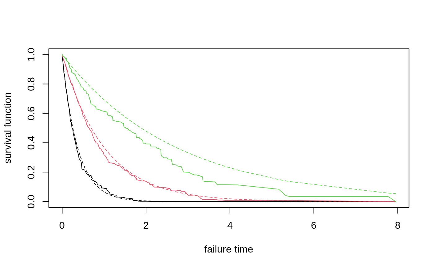
# \donttest{
# Train a standard survival forest.
n <- 2000
p <- 5
X <- matrix(rnorm(n * p), n, p)
failure.time <- exp(0.5 * X[, 1]) * rexp(n)
censor.time <- 2 * rexp(n)
Y <- pmin(failure.time, censor.time)
D <- as.integer(failure.time <= censor.time)
# Save computation time by constraining the event grid by discretizing (rounding) continuous events.
s.forest <- survival_forest(X, round(Y, 2), D)
# Or do so more flexibly by defining your own time grid using the failure.times argument.
# grid <- seq(min(Y[D==1]), max(Y[D==1]), length.out = 150)
# s.forest <- survival_forest(X, Y, D, failure.times = grid)

# Predict using the forest.
X.test <- matrix(0, 3, p)
X.test[, 1] <- seq(-2, 2, length.out = 3)
s.pred <- predict(s.forest, X.test)

# Plot the survival curve.
plot(NA, NA, xlab = "failure time", ylab = "survival function",
     xlim = range(s.pred$failure.times),
     ylim = c(0, 1))
for(i in 1:3) {
  lines(s.pred$failure.times, s.pred$predictions[i,], col = i)
  s.true = exp(-s.pred$failure.times / exp(0.5 * X.test[i, 1]))
  lines(s.pred$failure.times, s.true, col = i, lty = 2)
}

# Predict on out-of-bag training samples.
s.pred <- predict(s.forest)

# Compute OOB concordance based on the mortality score in Ishwaran et al. (2008).
s.pred.nelson.aalen <- predict(s.forest, prediction.type = "Nelson-Aalen")
chf.score <- rowSums(-log(s.pred.nelson.aalen$predictions))
if (require("survival", quietly = TRUE)) {
 concordance(Surv(Y, D) ~ chf.score, reverse = TRUE)
}
#> Call:
#> concordance.formula(object = Surv(Y, D) ~ chf.score, reverse = TRUE)
#> 
#> n= 2000 
#> Concordance= 0.6332 se= 0.00871
#> concordant discordant     tied.x     tied.y    tied.xy 
#>     842768     488263          0          0          0 
# }