Assessing overlap
Two common diagnostics to evaluate if the identifying assumptions behind grf hold is a propensity score histogram and covariance balance plot.
n <- 2000
p <- 10
X <- matrix(rnorm(n * p), n, p)
colnames(X) <- make.names(1:p)

W <- rbinom(n, 1, 0.4 + 0.2 * (X[, 1] > 0))
Y <- pmax(X[, 1], 0) * W + X[, 2] + pmin(X[, 3], 0) + rnorm(n)
cf <- causal_forest(X, Y, W)
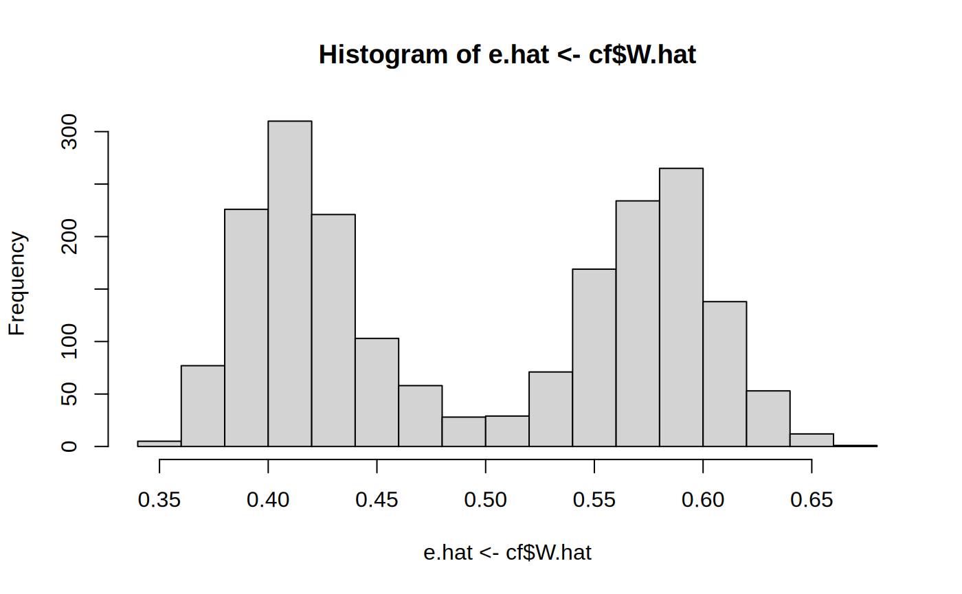
The overlap assumption requires a positive probability of treatment for each \(X_i\). We should not be able to deterministically decide the treatment status of an individual based on its covariates, meaning none of the estimated propensity scores should be close to one or zero. One can check this with a histogram:
hist(e.hat <- cf$W.hat)
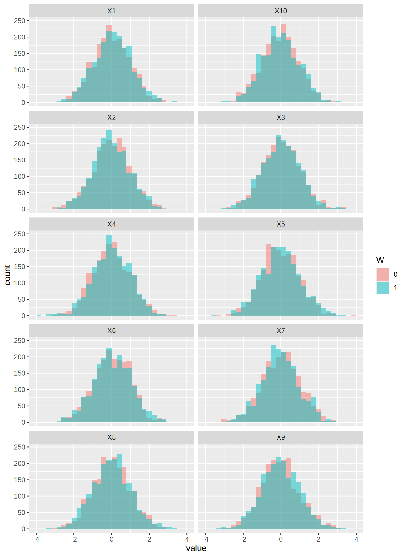
One can also check that the covariates are balanced across the treated and control group by plotting the inverse-propensity weighted histograms of all samples, overlaid here for each feature (done with ggplot2 which supports weighted histograms):
IPW <- ifelse(W == 1, 1 / e.hat, 1 / (1 - e.hat))

plot.df <- data.frame(value = as.vector(X),
                      variable = colnames(X)[rep(1:p, each = n)],
                      W = as.factor(W),
                      IPW = IPW)

ggplot(plot.df, aes(x = value, weight = IPW, fill = W)) +
  geom_histogram(alpha = 0.5, position = "identity", bins = 30) +
  facet_wrap( ~ variable, ncol = 2)
Assessing fit
The forest summary function test_calibration
can be used to asses a forest’s goodness of fit. A coefficient of 1 for
mean.forest.prediction suggests that the mean forest
prediction is correct and a coefficient of 1 for
differential.forest.prediction suggests that the forest has
captured heterogeneity in the underlying signal.
test_calibration(cf)
#>
#> Best linear fit using forest predictions (on held-out data)
#> as well as the mean forest prediction as regressors, along
#> with one-sided heteroskedasticity-robust (HC3) SEs:
#>
#>                                Estimate Std. Error t value    Pr(>t)
#> mean.forest.prediction          1.01570    0.13296  7.6393 1.683e-14 ***
#> differential.forest.prediction  1.19482    0.10324 11.5734 < 2.2e-16 ***
#> ---
#> Signif. codes:  0 '***' 0.001 '**' 0.01 '*' 0.05 '.' 0.1 ' ' 1
This exercise and function is motivated by earlier developments in the econometrics literature. A more intuitive exercise is to look at subgroup ATEs where the subgroups are formed according to low or high CATE predictions (Athey & Wager, 2019). While this approach may give some qualitative insight into heterogeneity, the grouping is naive, because the doubly robust scores used to determine subgroups are not independent of the scores used to estimate those group ATEs.
The RATE function automates this exercise over all possible subgroups using the quantiles of the CATE predictions. If we use separate data to fit CATE models and estimate RATE metrics, we obtain a test statistic with expectation zero under no heterogeneity, which can be used to construct confidence intervals for the presence of treatment effect heterogeneity. For more details on this preferred approach, please see this vignette.
Athey et al. (2017) suggests a bias measure to gauge how much work the propensity and outcome models have to do to get an unbiased estimate, relative to looking at a simple difference-in-means: \(bias(x) = (e(x) - p) \times (p(\mu(0, x) - \mu_0) + (1 - p) (\mu(1, x) - \mu_1)\).
tau.hat <- predict(cf)$predictions

p <- mean(W)
Y.hat.0 <- cf$Y.hat - e.hat * tau.hat
Y.hat.1 <- cf$Y.hat + (1 - e.hat) * tau.hat

bias <- (e.hat - p) * (p * (Y.hat.0 - mean(Y.hat.0))  + (1 - p) * (Y.hat.1 - mean(Y.hat.1)))
Scaled by the standard deviation of the outcome:
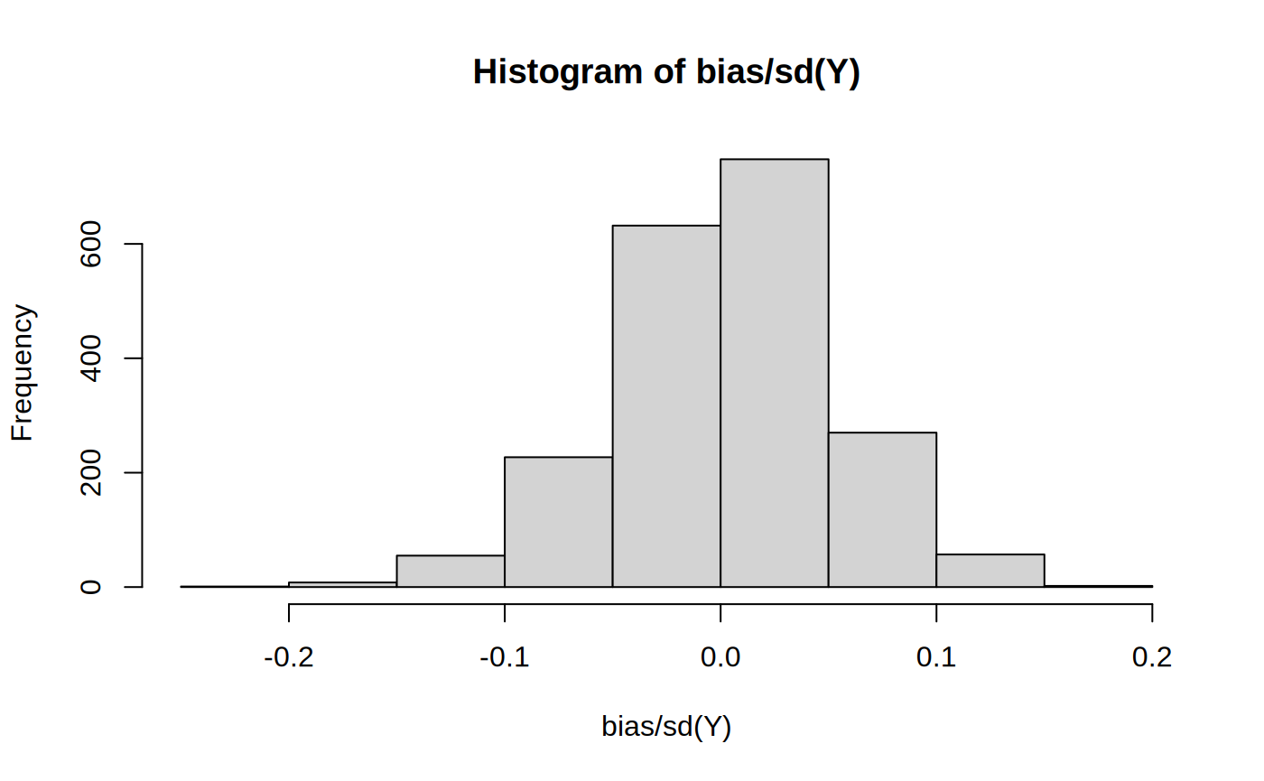
See Athey et al. (2017) section D for more details.
References
Athey, Susan and Stefan Wager. Estimating Treatment Effects with Causal Forests: An Application. Observational Studies, 5, 2019. (arxiv)
Athey, Susan, Guido Imbens, Thai Pham, and Stefan Wager. Estimating average treatment effects: Supplementary analyses and remaining challenges. American Economic Review, 107(5), May 2017: 278-281. (arxiv)