Policy learning via optimal decision trees • grf

library(grf)
library(policytree)

Using GRF it is possible to non-parametrically estimate a CATE function \(\hat \tau(\cdot)\), then use this as a treatment assignment policy, by for example treating units where the predictions \(\hat \tau(X_i)\) are positive. Let’s denote our policy by the symbol \(\pi\), which is a function that takes as input covariates \(X_i\) describing characteristics of a unit and outputs a treatment decision where \(0\) means don’t treat and \(1\) treat, i.e.

\[ \pi(\cdot) \mapsto \{0, 1\} \]

If we are using our estimated CATEs to assign treatment we may express \(\pi\) simply as \(\pi(X_i) = 1(\hat \tau(X_i) > 0)\). The vignette on Qini curves gives some examples of metrics one can construct on a held-out test set in order to evaluate this policy, as well as how to incorporate budget constraints.

In some settings, assigning treatment in this manner may be undesirable. Consider for example a welfare program that gives people job training skills. Deciding who to assign this program to based on a complicated black-box CATE function may be undesirable if policymakers want transparent criteria for who should be eligible for the program. Likewise, it may be problematic for potential recipients to learn they were denied a beneficial job training program solely because a black-box algorithm predicted they would not benefit sufficiently. In settings like these, we are interested in interpretable policies. I.e., we want a simple rule that looks at a unit’s characteristics \(X_i\) and gives a treatment decision. An example could be “Alice is assigned treatment because she is under 25 and lives in a disadvantaged neighborhood”. An example of such an interpretable policy would be the policy embedded in a shallow decision tree.

Tree-based treatment assignment rules

In order to learn a policy \(\pi\) from experimental or observational data, we need an efficient scoring rule, and an algorithm to find trees. The approach where we use “doubly robust” scoring and decision trees that optimize empirical welfare, is implemented in the package policytree. In order to learn a good shallow decision tree it is important to learn the branching decisions right at each level. Typical approaches to decision tree learning are based on greedy criteria (such as “CART”) and may not necessarily learn globally optimal branching decisions, the policytree package takes a tree learning approach that is more computationally involved but finds a globally optimal decision tree.¹

The brief example below demonstrates learning a depth-2 tree using doubly robust scores obtained from a causal forest. The function policy_tree and double_robust_scores belong to the policytree package.

# Fit a causal forest.
n <- 15000
p <- 5
X <- round(matrix(rnorm(n * p), n, p), 2)
W <- rbinom(n, 1, 1 / (1 + exp(X[, 3])))
tau <- 1 / (1 + exp((X[, 1] + X[, 2]) / 2)) - 0.5
Y <- X[, 3] + W * tau + rnorm(n)
c.forest <- causal_forest(X, Y, W)

# Compute doubly robust scores.
# (In observational settings it is usually a good idea to plot the estimated propensity
# scores (`hist(c.forest$W.hat)`) to ensure we have sufficient overlap)
dr.scores <- double_robust_scores(c.forest)
head(dr.scores)
#>         control    treated
#> [1,] -0.1894867  0.6539203
#> [2,]  0.2069720  2.2627534
#> [3,] -0.4586539 -0.6450377
#> [4,]  0.9696632 -1.2263088
#> [5,]  1.9203896  0.6905221
#> [6,] -3.5035332 -0.2376621

# Fit a depth-2 tree on the doubly robust scores.
tree <- policy_tree(X, dr.scores, depth = 2)

# Print and plot the tree - action 1 corresponds to control, and 2 treated.
print(tree)
#> policy_tree object 
#> Tree depth:  2 
#> Actions:  1: control 2: treated 
#> Variable splits: 
#> (1) split_variable: X1  split_value: -0.73 
#>   (2) split_variable: X2  split_value: 1.42 
#>     (4) * action: 2 
#>     (5) * action: 1 
#>   (3) split_variable: X2  split_value: -0.36 
#>     (6) * action: 2 
#>     (7) * action: 1
plot(tree)

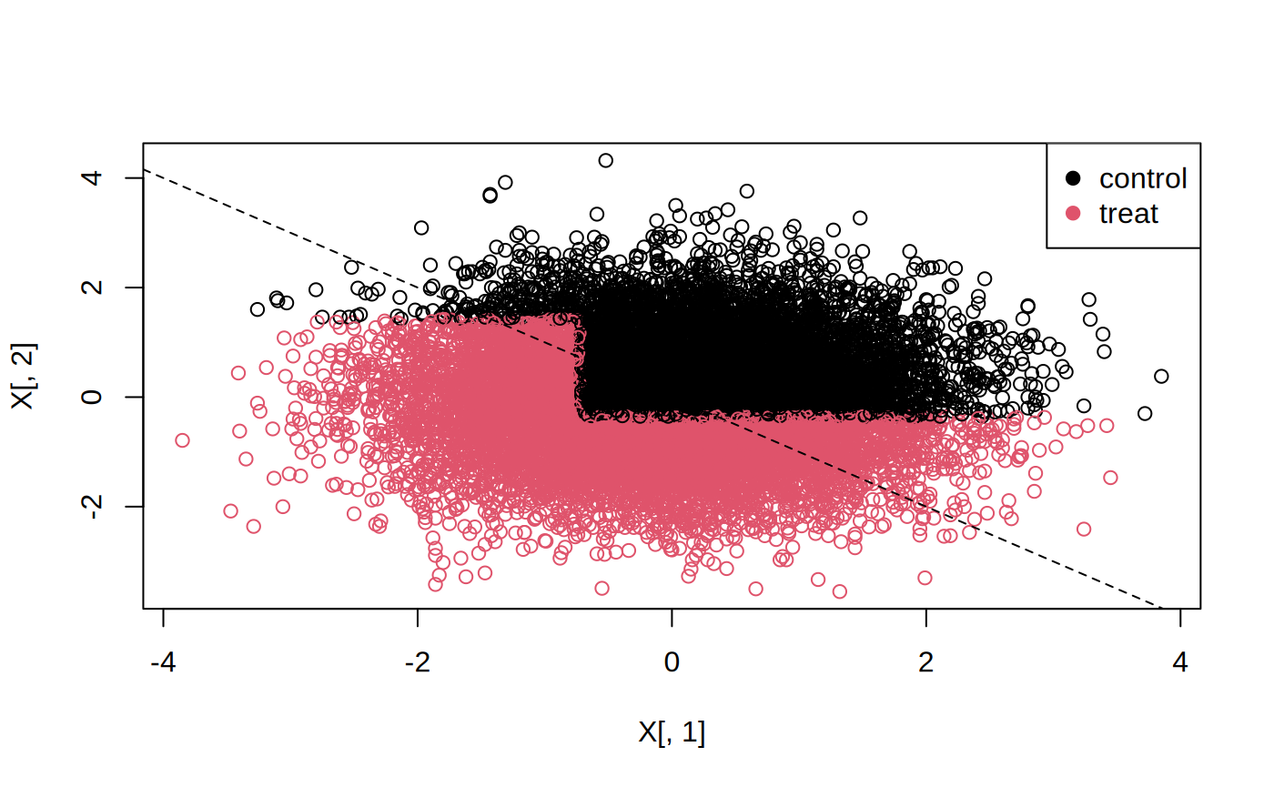
The 45-degree line in the following plot separates units with a negative effect (above the line), and a positive effect (below the line).

# Predict the treatment assignment {1, 2} for each sample.
predicted <- predict(tree, X)
plot(X[, 1], X[, 2], col = predicted)
legend("topright", c("control", "treat"), col = c(1, 2), pch = 19)
abline(0, -1, lty = 2)

Alternatively, predict can return the leaf node each sample falls into, which we can use to calculate statistics, such as average treatment effects, for each group (note that to avoid overfitting, statistics like these should be computed on a held-out test set separate from the one used for learning the policy, and can thus serve as a practical way do to train/test evaluation of a fit policy).

node.id <- predict(tree, X, type = "node.id")

# The value of all arms (along with SEs) by each leaf node.
values <- aggregate(dr.scores, by = list(leaf.node = node.id),
                    FUN = function(x) c(mean = mean(x), se = sd(x) / sqrt(length(x))))
print(values, digits = 2)
#>   leaf.node control.mean control.se treated.mean treated.se
#> 1         4       -0.105      0.034        0.178      0.034
#> 2         5        0.169      0.108        0.044      0.100
#> 3         6       -0.020      0.028        0.071      0.029
#> 4         7        0.019      0.022       -0.159      0.022

For more statistical details please see the chapter on Policy Learning in these lecture notes.

A description of the tree search algorithm is given in this paper.↩︎