library(grf)
This vignette gives a brief overview of strategies to evaluate CATE estimators via Rank-Weighted Average Treatment Effects (RATEs) that avoids a single training and evaluation split. We’re demonstrating the use of causal forest to detect heterogeneity via the RATE when using observational or experimental data with a binary treatment assignment and describe two proposals: a sequential fold estimation procedure and a heuristic for one-sided tests based on out-of-bag estimates.
Cross-fold estimation of RATE metrics
As covered in this vignette, RATE metrics can be used as a test for the presence of treatment heterogeneity. A common use case is to use a training set to obtain estimates of the conditional average treatment effect (CATE) and then evaluate these on a held-out test set using the RATE. Concretely, on a training set we can obtain some estimated CATE function \(\hat \tau(\cdot)\), then on a test we can obtain an estimate of the RATE, then form a test for whether we detect heterogeneity via:
\(H_0\): RATE \(=0\) (No heterogeneity detected by \(\hat \tau(\cdot)\))
\(H_A\): RATE \(\neq 0\).
RATE metrics satisfy a central-limit theorem and motivate a simple \(t\)-test of this hypothesis using
\[ t = \frac{\widehat{RATE}}{\sqrt{Var(\widehat{RATE})}}. \]
Using a confidence level \(\alpha\) of 5%, we reject \(H_0\) if the \(p\)-value \(2\Phi(-|t|)\) is less than 5%.
A drawback of this approach is that we are only utilizing a subset of our data to train a CATE estimator. In regimes with small sample sizes and hard-to-detect heterogeneity, this can be inconvenient. One appealing alternative could be to use cross-fold estimation, where we divide the data into \(K\) folds and then alternate which subset we use for training a CATE estimator and which subset we use to estimate the RATE. The figure below illustrates the case when using \(K=5\) folds: fit a CATE estimator on the blue sample, and evaluate the RATE on the red sample.
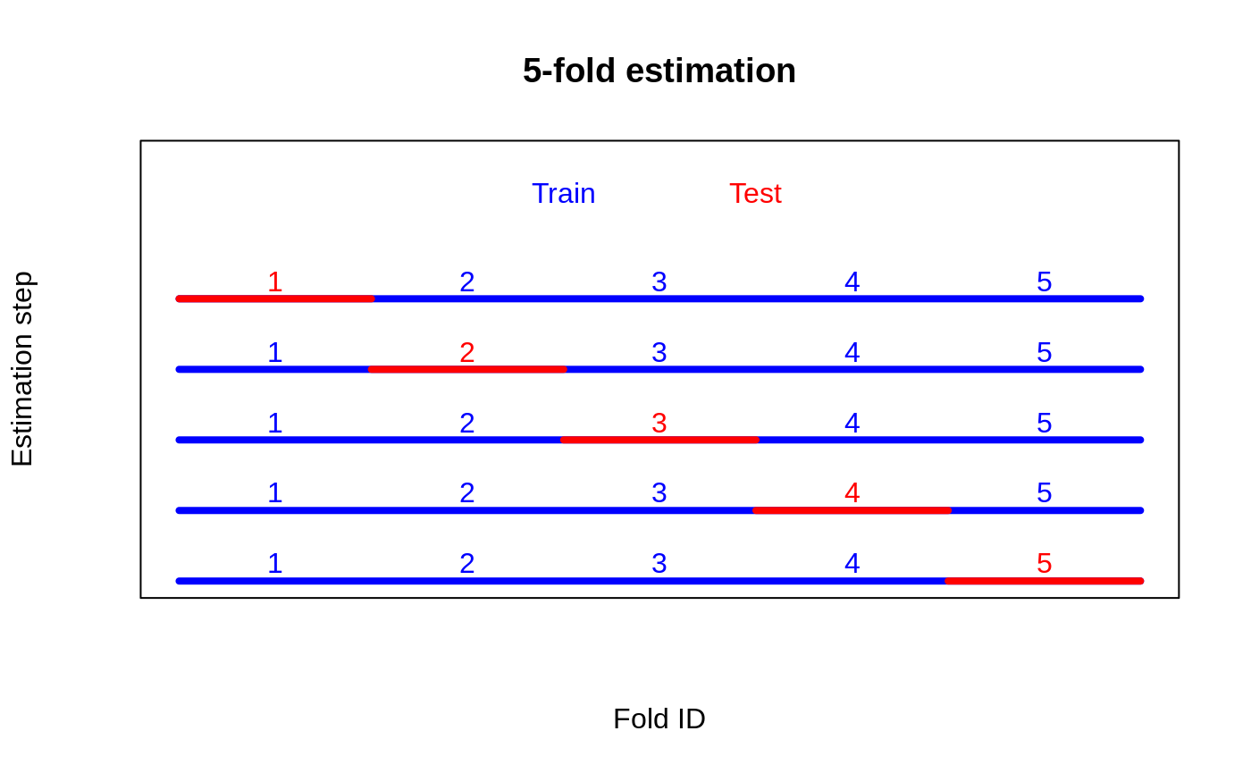
This strategy would give us 5 RATE estimates along with 5 \(t\)-values, and the hope would be that in aggregating these we are increasing our ability (power) to detect heterogeneity. On their own, each of these \(t\)-values serves as a valid test. The problem with aggregating them is that they are not independent, as the overlapping fold construction induces correlation.
We can see this play out in a simple simulation exercise. Below we define a simple function that splits the data into 5 folds, forms a RATE estimate and \(t\)-value on each fold, and then compute a \(p\)-value by aggregating the test statistics.
# Estimate RATE on K random folds to get K t-statistics, then return a p-value
# for H0 using the sum of these t-values.
rate_cv_naive = function(X, Y, W, num.folds = 5) {
  fold.id = sample(rep(1:num.folds, length = nrow(X)))
  samples.by.fold = split(seq_along(fold.id), fold.id)

  t.statistics = c()

  # Form AIPW scores for estimating RATE
  nuisance.forest = causal_forest(X, Y, W)
  DR.scores = get_scores(nuisance.forest)

  for (k in 1:num.folds) {
    train = unlist(samples.by.fold[-k])
    test = samples.by.fold[[k]]

    cate.forest = causal_forest(X[train, ], Y[train], W[train])

    cate.hat.test = predict(cate.forest, X[test, ])$predictions

    rate.fold = rank_average_treatment_effect.fit(DR.scores[test], cate.hat.test)
    t.statistics = c(t.statistics, rate.fold$estimate / rate.fold$std.err)
  }

  p.value.naive = 2 * pnorm(-abs(sum(t.statistics) / sqrt(num.folds)))

  p.value.naive
}
Next, we simulate synthetic data with no treatment heterogeneity, and form a Monte Carlo estimate of our naive procedure’s rejection probability, using a 5% confidence level:
res = t(replicate(500, {
  n = 1500
  p = 5
  X = matrix(rnorm(n * p), n, p)
  W = rbinom(n, 1, 0.5)
  Y = pmin(X[, 3], 0) + rnorm(n)

  pval.naive = rate_cv_naive(X, Y, W)

  c(
    reject = pval.naive <= 0.05
  )
}))
paste("Rejection rate:", mean(res) * 100, "%")
#> [1] "Rejection rate: 16.8 %"
At a 5% level, any test with a rejection rate above 5% is an invalid test.
Sequential cross-fold estimation
It turns out, however, that there exists a simple algorithmic fix that can address the shortcomings of naive cross-fold validation. This approach, which we call sequential cross-fold estimation, breaks up the correlation between RATE metrics across folds by only using training folds in sequential order. As illustrated in the figure below, this strategy will give us \(K - 1\) separate \(t\)-values.
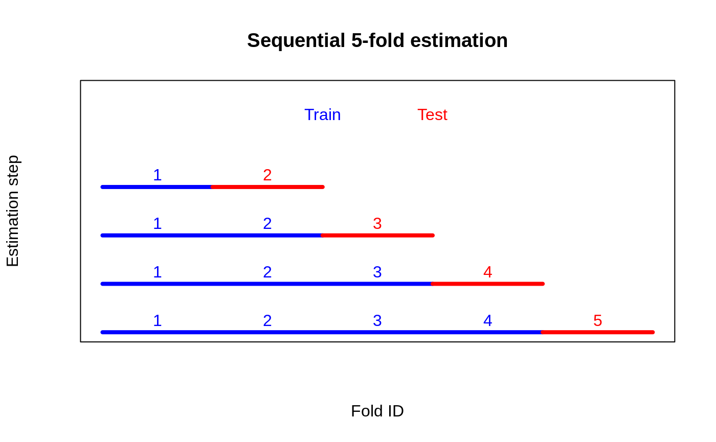
This construction is going to make our \(t\)-values satisfy a martingale property and allow for valid aggregation (Luedtke & van der Laan (2016), and Wager (2024)). The steps are:
Randomly split the data into \(k=1,\ldots,K\) evenly sized folds.
-
For each fold \(k=2,\ldots,K\):
Obtain an estimated CATE function using \(\color{blue}{\text{training}}\) data from folds \(1,\ldots,k-1\).
Form a RATE estimate using data from the \(k\)-th \(\color{red}{\text{test}}\) fold and compute a \(t\)-statistic.
Aggregate the \(K-1\) different \(t\)-statistics and use this as a final test statistic.
This procedure is coded in the simple function below.
# Estimate RATE on K-1 random sequential folds to get K-1 t-statistics, then return a p-value
# for H0 using the sum of these t-values
rate_sequential = function(X, Y, W, num.folds = 5) {
  fold.id = sample(rep(1:num.folds, length = nrow(X)))
  samples.by.fold = split(seq_along(fold.id), fold.id)

  t.statistics = c()

  # Form AIPW scores for estimating RATE
  nuisance.forest = causal_forest(X, Y, W)
  DR.scores = get_scores(nuisance.forest)

  for (k in 2:num.folds) {
    train = unlist(samples.by.fold[1:(k - 1)])
    test = samples.by.fold[[k]]

    cate.forest = causal_forest(X[train, ], Y[train], W[train])

    cate.hat.test = predict(cate.forest, X[test, ])$predictions

    rate.fold = rank_average_treatment_effect.fit(DR.scores[test], cate.hat.test)
    t.statistics = c(t.statistics, rate.fold$estimate / rate.fold$std.err)
  }

  p.value = 2 * pnorm(-abs(sum(t.statistics) / sqrt(num.folds - 1)))

  p.value
}
If we repeat the check on data with no heterogeneity we can see this construction gives us the correct rejection rate (within the error tolerance of our Monte Carlo repetitions):
res = t(replicate(500, {
  n = 1500
  p = 5
  X = matrix(rnorm(n * p), n, p)
  W = rbinom(n, 1, 0.5)
  Y = pmin(X[, 3], 0) + rnorm(n)

  pval.sequential = rate_sequential(X, Y, W)

  c(
    reject.sequential = pval.sequential <= 0.05
  )
}))
paste("Rejection rate:", mean(res) * 100, "%")
#> [1] "Rejection rate: 5.4 %"
Now that we have a valid test for treatment heterogeneity that uses several folds, let’s try it out on a simulated example and examine how it performs in detecting treatment effect heterogeneity. The baseline we are comparing with is sample splitting, which is proven to be valid in the RATE paper, but which has potentially lower power since we are only using a fraction of our data for validation.
Below we generate data from synthetic observational data (Setup A in Nie & Wager (2021)) where treatment effect heterogeneity is hard to detect. Remember, in this case, we want our test to reject \(H_0\) of no heterogeneity.
res = t(replicate(500, {
  # Simulate synthetic data with "weak" treatment heterogeneity
  n = 2500
  p = 5
  data = generate_causal_data(n, p, sigma.tau = 0.15, sigma.noise = 1, dgp = "nw1")
  X = data$X
  Y = data$Y
  W = data$W

  pval.sequential = rate_sequential(X, Y, W)

  # Compare with a single train/test split
  train = sample(n, n / 2)
  test = -train
  cf.train = causal_forest(X[train,], Y[train], W[train])
  cf.test = causal_forest(X[test,], Y[test], W[test])
  rate = rank_average_treatment_effect(cf.test, predict(cf.train, X[test, ])$predictions)
  tstat.split = rate$estimate / rate$std.err
  pval.split = 2 * pnorm(-abs(tstat.split))

  c(
    reject.sequential = pval.sequential <= 0.05,
    reject.split = pval.split <= 0.05
  )
}))
colMeans(res) * 100
#> reject.sequential    reject.split
#> 56.6                 47.0
Reassuringly, in this example, cross-fold estimation is able to improve power to detect treatment heterogeneity over our baseline.
Heuristic: out-of-bag estimation with one-sided tests
The fundamental challenge with estimating CATEs and evaluating the presence of heterogeneity using the same data is overfitting: we’re simply constrained by the fact that we can’t simply estimate and evaluate something using the same data set. We saw that naive cross-fold estimation did not overcome this challenge due to between-fold correlations (that biases our estimate downwards). A heuristic to salvage this naive aggregation is to use one-sided \(p\)-values. If we are willing to commit to a one-sided test, for example, RATE \(>0\), this can serve as a useful strategy.
Random forests, however, have a more computationally efficient alternative to simple cross-fold estimation. The forest-native version of leave-one-out estimation is out-of-bag (OOB) estimation. For a given unit \(i\), these are estimates that are formed using all the trees in the random forest grown on subsamples that does not include the \(i\)-th unit. OOB-estimated RATEs paired with one-sided tests can serve as a useful heuristic when we want to use all our data to fit and evaluate heterogeneity.
In the example below we compare a two-sided test for RATE \(\neq 0\) with a one-sided test for RATE \(>0\) at a 5% level.
res = t(replicate(500, {
  n = 1500
  p = 5
  X = matrix(rnorm(n * p), n, p)
  W = rbinom(n, 1, 0.5)
  Y = pmin(X[, 3], 0) + rnorm(n)

  c.forest = causal_forest(X, Y, W)
  tau.hat.oob = predict(c.forest)$predictions
  rate.oob = rank_average_treatment_effect(c.forest, tau.hat.oob)

  t.stat.oob = rate.oob$estimate / rate.oob$std.err
  # Compute a two-sided p-value Pr(>|t|)
  p.val = 2 * pnorm(-abs(t.stat.oob))
  # Compute a one-sided p-value Pr(>t)
  p.val.onesided = pnorm(t.stat.oob, lower.tail = FALSE)

  c(
    reject.oob = p.val <= 0.05,
    reject.oob.onesided = p.val.onesided <= 0.05
  )
}))
colMeans(res) * 100
#> reject.oob reject.oob.onesided
#> 30.4                 4.0
We see that the one-sided test gives us a correct rejection rate of a null effect.
If we repeat the simple power exercise from above, we see that we achieve power essentially the same as sequential aggregation.
res = t(replicate(500, {
  # Simulate synthetic data with "weak" treatment heterogeneity
  n = 2500
  p = 5
  data = generate_causal_data(n, p, sigma.tau = 0.15, sigma.noise = 1, dgp = "nw1")
  X = data$X
  Y = data$Y
  W = data$W

  c.forest = causal_forest(X, Y, W)
  tau.hat.oob = predict(c.forest)$predictions
  rate.oob = rank_average_treatment_effect(c.forest, tau.hat.oob)
  t.stat.oob = rate.oob$estimate / rate.oob$std.err
  # Compute a one-sided p-value Pr(>t)
  p.val.onesided = pnorm(t.stat.oob, lower.tail = FALSE)

  c(
    reject.oob.onesided = p.val.onesided <= 0.05
  )
}))
mean(res) * 100
#> [1] 54.0
References
Chernozhukov, Victor, Mert Demirer, Esther Duflo, and Ivan Fernandez-Val. Generic machine learning inference on heterogeneous treatment effects in randomized experiments, with an application to immunization in India. Econometrica, forthcoming.
Luedtke, Alexander R., and Mark J. van der Laan. Statistical inference for the mean outcome under a possibly non-unique optimal treatment strategy. Annals of Statistics 44(2), 2016.
Nie, Xinkun, and Stefan Wager. Quasi-oracle estimation of heterogeneous treatment effects. Biometrika 108(2), 2021.
Wager, Stefan. Sequential Validation of Treatment Heterogeneity. arXiv preprint arXiv:2405.05534 (arxiv)
Appendix: Median aggregation of p-values
One possible solution to salvage rate_cv_naive is to
keep the traditional \(K\)-fold
construction, but change the way we aggregate \(t\)-statistics for each fold. This is the
strategy Chernozhukov et al. (2024) pursue. If instead of computing a
\(p\)-value based on aggregated \(t\)-statistics, we take a median of \(p\)-values based on each \(t\)-statistic, we get a valid test.
# This function does the same thing as `rate_naive`, except it returns
# the median p-value.
rate_cv_median = function(X, Y, W, num.folds = 5) {
  fold.id = sample(rep(1:num.folds, length = nrow(X)))
  samples.by.fold = split(seq_along(fold.id), fold.id)

  t.statistics = c()

  nuisance.forest = causal_forest(X, Y, W)
  DR.scores = get_scores(nuisance.forest)

  for (k in 1:num.folds) {
    train = unlist(samples.by.fold[-k])
    test = samples.by.fold[[k]]

    cate.forest = causal_forest(X[train, ], Y[train], W[train])

    cate.hat.test = predict(cate.forest, X[test, ])$predictions

    rate.fold = rank_average_treatment_effect.fit(DR.scores[test], cate.hat.test)
    t.statistics = c(t.statistics, rate.fold$estimate / rate.fold$std.err)
  }

  p.value.median = median(2 * pnorm(-abs(t.statistics)))

  p.value.median
}
This construction gives us a valid rejection rate using a 5% confidence value, but is quite conservative:
res = t(replicate(500, {
  n = 1500
  p = 5
  X = matrix(rnorm(n * p), n, p)
  W = rbinom(n, 1, 0.5)
  Y = pmin(X[, 3], 0) + rnorm(n)

  rate.cv.median = rate_cv_median(X, Y, W)

  c(
    reject.median = rate.cv.median <= 0.05
  )
}))
paste("Rejection rate:", mean(res) * 100, "%")
#> [1] "Rejection rate: 0.2 %"
If we repeat the power simulation from above, this algorithm does
unfortunately not yield higher power than sample splitting. A drawback
of this approach is that if all the \(t\)-statistics are positive, but not
significant on their own, then rate_sequential can take
this into account, while rate_cv_median cannot.
res = t(replicate(500, {
  # Simulate synthetic data with "weak" treatment heterogeneity
  n = 2500
  p = 5
  data = generate_causal_data(n, p, sigma.tau = 0.15, sigma.noise = 1, dgp = "nw1")
  X = data$X
  Y = data$Y
  W = data$W

  pval.median = rate_cv_median(X, Y, W)

  # Compare with sample splitting
  train = sample(n, n / 2)
  test = -train
  cf.train = causal_forest(X[train,], Y[train], W[train])
  cf.test = causal_forest(X[test,], Y[test], W[test])
  rate = rank_average_treatment_effect(cf.test, predict(cf.train, X[test, ])$predictions)
  tstat.split = rate$estimate / rate$std.err
  pval.split = 2 * pnorm(-abs(tstat.split))

  c(
    reject.median = pval.median <= 0.05,
    reject.split = pval.split <= 0.05
  )
}))
colMeans(res) * 100
#> reject.median  reject.split
#> 14.6          47.8