library(grf)
The following script demonstrates how to use GRF for heterogeneous treatment effect estimation. For examples of how to use other types of forests, please consult the R documentation on the relevant methods.
Generate data and train a causal forest
n <- 2000
p <- 10
X <- matrix(rnorm(n * p), n, p)
X.test <- matrix(0, 101, p)
X.test[, 1] <- seq(-2, 2, length.out = 101)

W <- rbinom(n, 1, 0.4 + 0.2 * (X[, 1] > 0))
Y <- pmax(X[, 1], 0) * W + X[, 2] + pmin(X[, 3], 0) + rnorm(n)
tau.forest <- causal_forest(X, Y, W)
tau.forest
#> GRF forest object of type causal_forest
#> Number of trees: 2000
#> Number of training samples: 2000
#> Variable importance:
#>     1     2     3     4     5     6     7     8     9    10
#> 0.688 0.032 0.044 0.043 0.033 0.029 0.031 0.028 0.030 0.042
Estimate treatment effects for the training data using out-of-bag prediction.
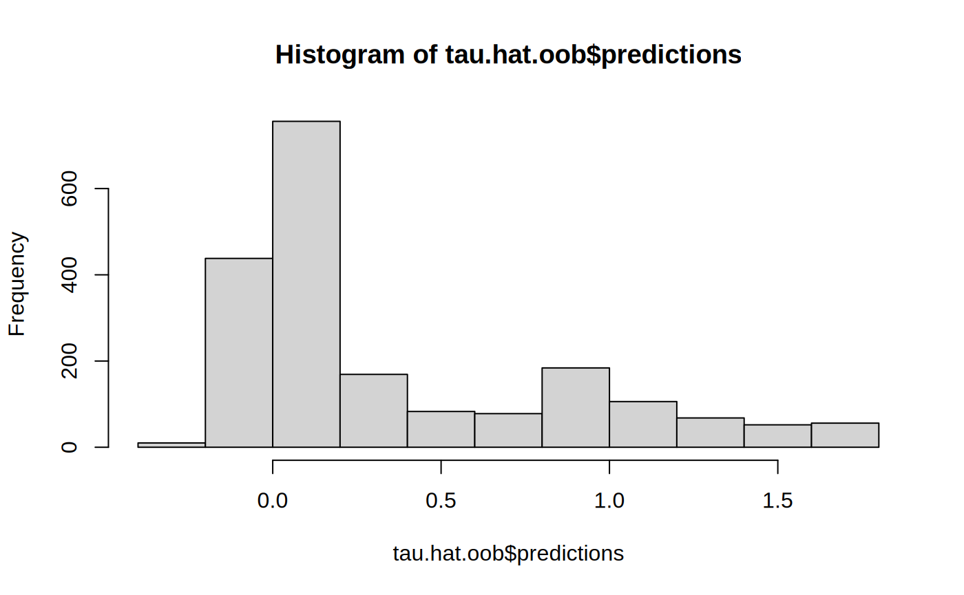
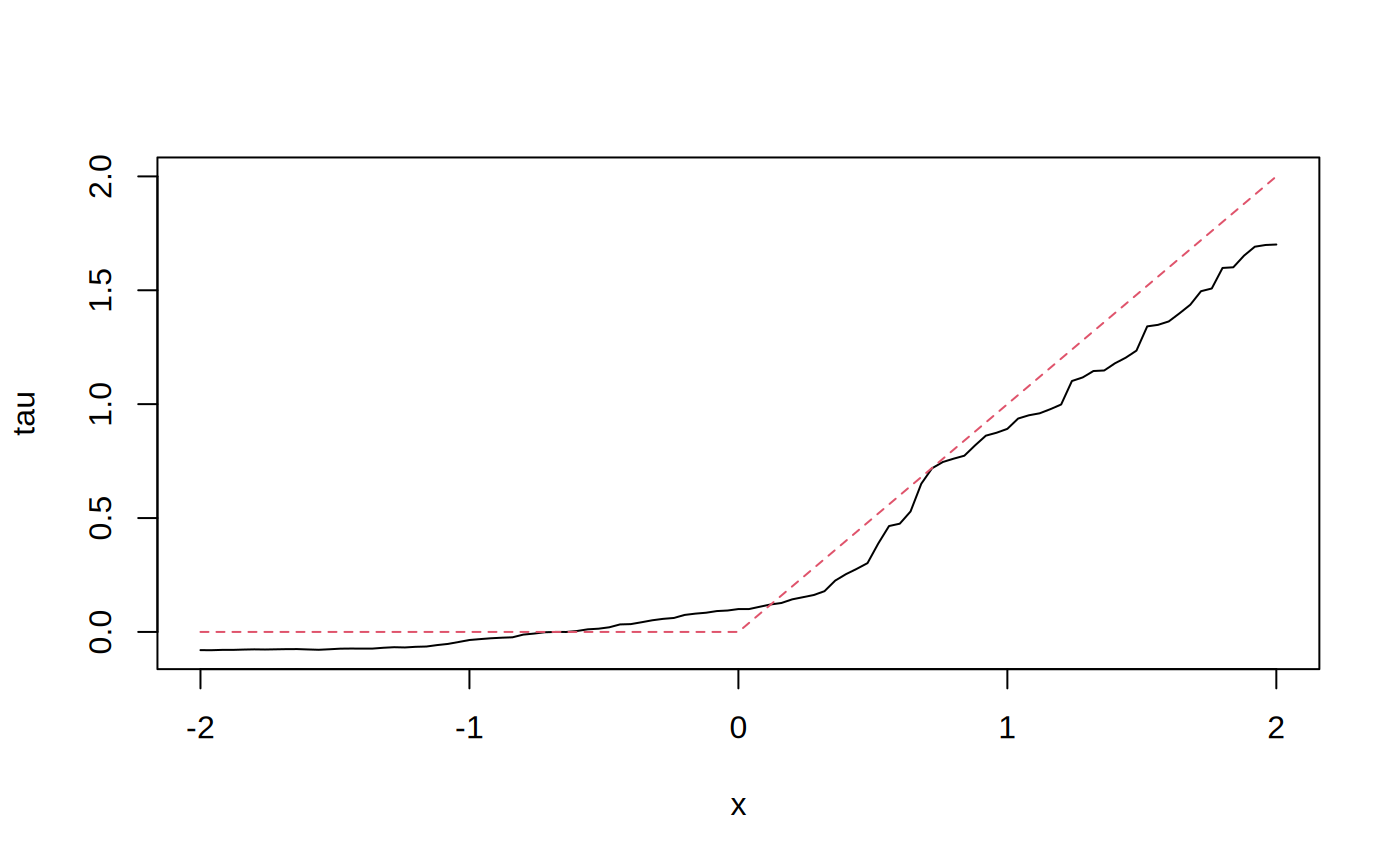
Estimate treatment effects for the test sample.
tau.hat <- predict(tau.forest, X.test)
plot(X.test[, 1], tau.hat$predictions, ylim = range(tau.hat$predictions, 0, 2), xlab = "x", ylab = "tau", type = "l")
lines(X.test[, 1], pmax(0, X.test[, 1]), col = 2, lty = 2)
Estimate the conditional average treatment effect on the full sample (CATE).
average_treatment_effect(tau.forest, target.sample = "all")
#>   estimate    std.err
#> 0.36644474 0.05003444
Estimate the conditional average treatment effect on the treated sample (CATT).
average_treatment_effect(tau.forest, target.sample = "treated")
#>   estimate    std.err
#> 0.46023739 0.05156137
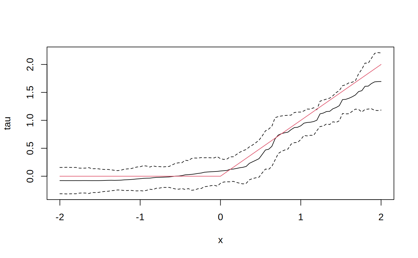
Add confidence intervals for heterogeneous treatment effects; growing more trees is now recommended.
tau.forest <- causal_forest(X, Y, W, num.trees = 4000)
tau.hat <- predict(tau.forest, X.test, estimate.variance = TRUE)
sigma.hat <- sqrt(tau.hat$variance.estimates)
plot(X.test[, 1], tau.hat$predictions, ylim = range(tau.hat$predictions + 1.96 * sigma.hat, tau.hat$predictions - 1.96 * sigma.hat, 0, 2), xlab = "x", ylab = "tau", type = "l")
lines(X.test[, 1], tau.hat$predictions + 1.96 * sigma.hat, col = 1, lty = 2)
lines(X.test[, 1], tau.hat$predictions - 1.96 * sigma.hat, col = 1, lty = 2)
lines(X.test[, 1], pmax(0, X.test[, 1]), col = 2, lty = 1)
In some examples, pre-fitting models for Y and W separately may be helpful (e.g., if different models use different covariates). In some applications, one may even want to get Y.hat and W.hat using a completely different method (e.g., boosting).
# Generate new data.
n <- 4000
p <- 20
X <- matrix(rnorm(n * p), n, p)
TAU <- 1 / (1 + exp(-X[, 3]))
W <- rbinom(n, 1, 1 / (1 + exp(-X[, 1] - X[, 2])))
Y <- pmax(X[, 2] + X[, 3], 0) + rowMeans(X[, 4:6]) / 2 + W * TAU + rnorm(n)

forest.W <- regression_forest(X, W, tune.parameters = "all")
W.hat <- predict(forest.W)$predictions

forest.Y <- regression_forest(X, Y, tune.parameters = "all")
Y.hat <- predict(forest.Y)$predictions

forest.Y.varimp <- variable_importance(forest.Y)

# Note: Forests may have a hard time when trained on very few variables
# (e.g., ncol(X) = 1, 2, or 3). We recommend not being too aggressive
# in selection.
selected.vars <- which(forest.Y.varimp / mean(forest.Y.varimp) > 0.2)

tau.forest <- causal_forest(X[, selected.vars], Y, W,
                            W.hat = W.hat, Y.hat = Y.hat,
                            tune.parameters = "all")
See if a causal forest succeeded in capturing heterogeneity by plotting the TOC and calculating a 95% CI for the AUTOC.
train <- sample(1:n, n / 2)
train.forest <- causal_forest(X[train, ], Y[train], W[train])
eval.forest <- causal_forest(X[-train, ], Y[-train], W[-train])
rate <- rank_average_treatment_effect(eval.forest,
                                      predict(train.forest, X[-train, ])$predictions)
plot(rate)
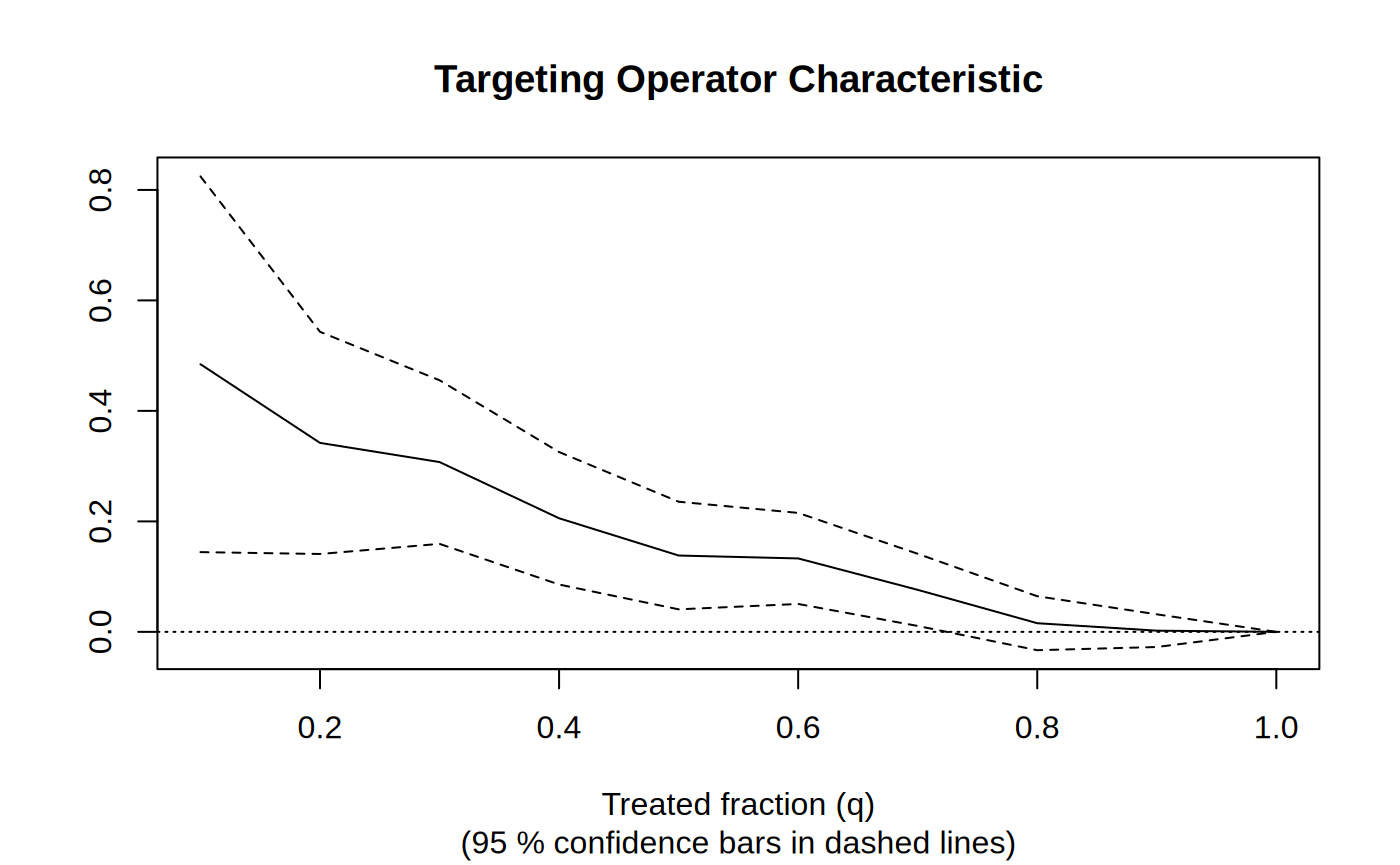
paste("AUTOC:", round(rate$estimate, 2), "+/", round(1.96 * rate$std.err, 2))
#> [1] "AUTOC: 0.2 +/ 0.1"
For more worked examples see the Tutorials section.