This vignette introduces forest-based causal inference using the
grf package for R. Generalized random forests
(Athey, Tibshirani, & Wager, 2019) extend Breiman (2001)’s random forest
to enable data-driven estimation of heterogeneity in causal parameters,
such as conditional average treatment effects under unconfoundedness. We
outline core functionality, including doubly robust estimation of
average treatment effects, best linear projections, tools for assessing
heterogeneity using TOC curves, evaluation of treatment rules via Qini
curves, and methods for learning interpretable tree-based policies. The
vignette contains two applied examples illustrating treatment effect
heterogeneity in practice. For further details, see the package
documentation and additional applied tutorials by Athey & Wager (2019), and Sverdrup,
Petukhova, & Wager (2024).
Vignette sections:
A grf guided tour
We describe how modern machine learning can flexibly control for confounding when estimating average treatment effects, how Breiman’s (2001) random forest can be adapted to target treatment effect heterogeneity, and how this approach extends to a broad class of settings, including instrumental variables and right-censored outcomes. Further info is provided in Athey & Wager (2019), Cui et al. (2023), Dandl et al. (2024), Friedberg et al. (2020), and Sverdrup et al. (2024). For a more detailed theoretical treatment, Wager (2024) provides a textbook-style discussion.
Machine learning for causal inference
Machine learning methods are designed for prediction. In causal applications, however, our goal is often inference rather than prediction. Although statistical estimation and statistical prediction are distinct tasks (Efron, 2020), predictive tools can support valid inference when used appropriately. This section outlines how modern machine learning, combined with ideas from semi-parametric statistics, can provide flexible and model-agnostic tools for causal inference.
Suppose we observe outcomes \(Y_i\), a binary treatment indicator \(W_i \in {0,1}\), and covariates \(X_i\). Our goal is to estimate the average treatment effect \(\tau = \text{E}[Y_i(1) - Y_i(0)]\). In an observational study, we might run a regression \[ Y_i \sim \tau W_i + \beta X_i, \] and interpret \(\hat\tau\) as an estimate of the ATE. This interpretation relies on:
- \(W\) being unconfounded given \(X\) (e.g., Rosenbaum and Rubin, 1983).
- The confounders \(X\) having a linear effect on \(Y\).
- The treatment effect \(\tau\) being constant.
Assumption 1) is an identifying assumption and something we choose to live with depending on domain knowledge. Assumptions 2) and 3) are modeling choices that we may wish to relax.
Relaxing assumption 2). Instead of assuming linearity, consider the partially linear model \[ Y_i = \tau W_i + f(X_i) + \varepsilon_i, \quad \text{E}[\varepsilon_i \mid X_i, W_i] = 0, \] where \(f\) is an unknown function. The challenge is that \(f(X_i)\) is not specified.
Robinson (1988) shows that via the following intermediary objects, the propensity score \[ e(x) = \text{E}[W_i \mid X_i=x], \] and the conditional mean, \[ m(x) = \text{E}[Y_i \mid X_i = x] = f(x) + \tau e(x), \] we can rewrite the model in centered form: \[ Y_i - m(x) = \tau \Big(W_i - e(x)\Big) + \varepsilon_i. \] This means that \(\tau\) can be estimated by regressing the residualized outcome on the residualized treatment. Importantly, Robinson (1988) showed that this estimator is root-\(n\) consistent even if \(m(x)\) and \(e(x)\) are estimated more slowly. This robustness is often called orthogonality: small errors in nuisance estimates do not substantially bias the target parameter.
How do we flexibly estimate \(m(x)\)
and \(e(x)\)? These are standard
regression problems: predict \(Y_i\)
from \(X_i\), and \(W_i\) from \(X_i\). Modern machine learning methods,
such as boosting or random forests, are well suited for this task (James
et al., 2013). A
wrinkle is that directly plugging machine learning estimates into this
estimator can lead to bias due to regularization. A standard technique
in semi-parametric estimation is sample splitting, where separate data
subsets are used to train and evaluate these components. Cross-fitting,
alternating which folds are used for training and estimation, is a
common implementation (Chernozhukov et al., 2018; Zheng & van der
Laan, 2011).
In grf, out-of-bag predictions provide a
forest-native leave-one-out form of cross-fitting.
Relaxing assumption 3). Instead of assuming constant treatment effects, suppose treatment effects vary with covariates: \[ Y_i = \textcolor{red}{\tau(X_i)}W_i + f(X_i) + \varepsilon_i, \, \, \text{E}[\varepsilon_i \mid X_i, W_i] = 0, \] where \(\textcolor{red}{\tau(x)}\) is the conditional average treatment effect \(\text{E}[Y_i(1) - Y_i(0) \mid X_i = x]\). If we had access to a neighborhood \(\mathcal{N}(x)\) where \(\tau\) were approximately constant, we could proceed exactly as before, by performing a residual-on-residual regression on the samples belonging to \(\mathcal{N}(x)\), i.e.: \[ \tau(x) := \text{lm}\Biggl( Y_i - \hat m^{(-i)}(X_i) \sim W_i - \hat e^{(-i)}(X_i), \text{weights} = 1\{X_i \in \mathcal{N}(x) \}\Biggr), \] where \(^{{(-i)}}\) denotes out-of-bag estimates. Conceptually, causal forest estimates \(\tau(x)\) by running a locally weighted residual-on-residual regression using samples predicted to have similar treatment effects.
The key question is how to construct these weights. The next section reviews Breiman’s random forest and explains how it serves as an adaptive neighborhood finder.
Random forest as an adaptive neighborhood finder
Breiman’s random forest estimates the conditional mean \(\mu(x) = \text{E}[Y_i \mid X_i = x]\) in two phases:
Building phase: Grow \(B\) trees by greedily choosing covariate splits that maximize the squared difference in subgroup means \(n_L n_R (\bar y_L - \bar y_R)^2\).
Prediction phase: For a target sample \(x\), average the outcomes \(Y_i\) in the same terminal leaf \(L_b(x)\) across trees: \(\hat \mu(x) = \frac{1}{B} \sum\limits_{b=1}^{B} \sum\limits_{i=1}^{n} Y_i \dfrac{1\{Xi \in L_b(x)\}} {|L_b(x)|}\).
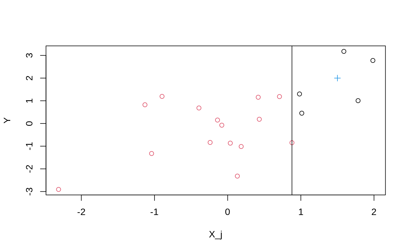
For a single tree and split, Figure 1 shows the chosen split point: the vertical line that maximizes the difference in leaf means. A target point \(x\) falls into one leaf, and prediction averages outcomes in that leaf. Repeating over trees and averaging yields the final estimate.
Rewriting the prediction as \[\begin{equation*} \begin{split} \hat \mu(x) & = \sum_{i=1}^{n} \frac{1}{B} \sum_{b=1}^{B} Y_i \frac{1\{X_i \in L_b(x)\}} {|L_b(x)|} \\ & = \sum_{i=1}^{n} Y_i \textcolor{magenta}{\alpha_i(x)}, \end{split} \end{equation*}\] shows that a random forest prediction is a weighted average of outcomes. The weights \(\textcolor{magenta}{\alpha_i(x)}\) reflect how often training sample \(i\) shares a leaf with \(x\). They can be interpreted as adaptive similarity weights. This weighting view of random forests appears frequently in statistical applications, see for example Zeileis, Hothorn & Hornik (2003).
Causal forests combines this forest weighting with Robinson’s approach:
Building phase: Choose splits that maximize the squared difference in estimated subgroup treatment effects, \(n_L n_R (\hat \tau_L - \hat \tau_R)^2\), where \(\hat\tau\) is computed via residual-on-residual regression.
Prediction phase: Use the resulting forest weights \(\textcolor{magenta}{\alpha(x)}\) to estimate \[ \tau(x) := \text{lm}\Biggl( Y_i - \hat m^{(-i)}(X_i) \sim W_i - \hat e^{(-i)}(X_i),~ \text{weights} = \textcolor{magenta}{\alpha_i(x)} \Biggr). \]
Thus, causal forest performs a forest-localized version of Robinson’s
regression. In causal_forest, the arguments
Y.hat and W.hat provide estimates of \(m(x)\) and \(e(x)\), by default obtained from separate
regression forests. If we are in a randomized setting where we know the
propensity score, we can simply supply these via the W.hat
argument. Robinson’s transformation also motivates a general loss
function for heterogeneous treatment effects (Nie & Wager, 2021), which
causal_forest uses to guide the selection of tuning
parameters.
The same idea extends beyond treatment effects and
residual-on-residual regressions. In the generalized random forest
framework, the forest is tailored to target heterogeneity in any
parameter defined by an estimating equation \(\psi_\theta(\cdot)\). Given an estimating
equation that identifies a parameter \(\theta\) without covariates,
grf then constructs weights \(\alpha(x)\) that yield covariate-specific
estimates \(\theta(x)\), using
Breiman’s random forest as a blueprint. For causal forests, this
estimating equation corresponds to Robinson’s regression.
Orthogonal estimating equations offers practical advantages by
separating the statistical tasks. Other forests, such as
instrumental_forest and
causal_survival_forest, use similar constructions. For
example, causal_survival_forest fits two separate survival
forests to construct right-censoring adjustments. These are then used to
construct an orthogonal estimating equation, and grf trains
a final random forest targeting heterogeneity in the treatment effect
parameter.
For computational and implementation reasons, grf does
not re-estimate the target parameter at every candidate split in the
building phase. Instead, it uses an influence-function-based
approximation computed once in the parent node. grf then
reuses the standard random forest machinery (Breiman-style tree growth
and regression-based splitting) but replaces the raw outcomes with
pseudo-outcomes derived from the orthogonal score. From an
implementation perspective, this means that new forest estimators can be
built by specifying the appropriate score and pseudo-outcome, while
leaving the underlying random forest algorithm unchanged.
Note: The target parameter \(\theta\) may be vector-valued. In that case, splits are based on the squared \(\ell_2\) distance \(n_L n_R \lVert \hat\theta_L - \hat\theta_R \rVert^2\), as in
grf’smulti_arm_causal_forestandlm_forest.
Efficiently estimating summaries of the CATEs
Robinson’s residual-on-residual approach is orthogonal, which makes it well suited for estimates that converge slowly. But what if we want summaries of \(\tau(x)\), such as the ATE or a best linear projection (BLP), that have guaranteed root-\(n\) rate of convergence along with exact confidence intervals?
Simply averaging the estimates \(\hat\tau(X_i)\) is not optimal: prediction errors are too large and do not cancel out. Robins, Rotnitzky & Zhao (1994) proposed the Augmented Inverse Probability Weighted (AIPW) estimator, which combines propensity scores and conditional mean estimates in a way that is robust to estimation errors in either component. It can be expressed as a one-step debiasing correction, taking the following form
\[ \hat \Gamma_i = \hat \tau^{(-i)}(X_i) + \frac{W_i - \hat e^{(-i)}(X_i)}{\hat e^{(-i)}(X_i)[1 - \hat e^{(-i)}(X_i)]} \Big(Y_i - \hat \mu^{(-i)}(X_i, W_i)\Big), \] where \(\mu(x, w) = E[Y_i \mid X_i = x, W_i = w]\) (this can be backed out from a causal forest fit). The forest-based ATE is then given by \[ \hat \tau_{\text{AIPW}} = \frac{1}{n} \sum_{i=1}^{n} \hat \Gamma_i. \]
This construction yields doubly robust estimating
equations and forms the basis of summary methods in grf,
including average_treatment_effect and
best_linear_projection. The associated doubly robust scores
\(\hat \Gamma_i\) are accessible
through the function get_scores. As a concrete example, the
ATE is an average of \(\hat
\Gamma_i\)’s, while the best linear projection is a regression of
the \(\hat \Gamma_i\)’s on a set of
covariates \(X_i\).
Assessing heterogeneity with TOC curves
Combined with techniques such as honesty and subsampling (Wager & Athey, 2018), the generalized random forest algorithm supports pointwise asymptotic guarantees. Results like these are reassuring, as they characterize the large-sample behavior of the forest. For practical purposes, however, there are more direct and transparent ways to assess whether meaningful heterogeneity is present in a given dataset.
A simple and pragmatic approach is train/test evaluation. We fit a CATE model on a training set, then on a held-out test set, we form subgroups based on predicted treatment effects and examine whether average treatment effects differ systematically across these groups. This approach is quite general: we may evaluate any machine-learned targeting function, including alternative effect measures, such as predicted risk or other quantities that may be aligned with treatment benefit in a given application. As long as higher values correspond to higher expected treatment gains, the same evaluation logic applies (for approaches that do not rely on a single train/test split, see, for example, Wager (2024)).
The rank_average_treatment_effect function provides an
automated implementation of this exercise by stratifying the test sample
according to all quantiles of the estimated targeting function. The
Targeting Operator Characteristic (TOC) curve (Yadlowsky et
al., 2024)
compares the average treatment effect among units with predicted CATEs
in the top \(q\)-th quantile to the
overall ATE. \[
\text{TOC}(q) = \text{E}[Y_i(1) - Y_i(0) \mid \text{Estimated CATE}(X_i)
\geq (1 - q)\text{-th quantile}] - \text{ATE}.
\] Given a trained evaluation forest, grf provides
doubly robust estimates of the TOC and the area under the TOC, along
with standard errors that enable a simple and valid \(t\)-test for the presence of heterogeneity.
Under the null of constant treatment effects, the area under the TOC
curve is zero in expectation.
A user can also supply two estimated CATEs or, more generally, two
targeting scores in order to compare prioritization strategies. The
rank_average_treatment_effect function then returns
estimates and confidence intervals for the difference in the area under
the TOC curves, which can be used to test whether the two targeting
scores differ significantly in their ability to prioritize units for
treatment.
Policy evaluation with Qini curves
We are often interested in data-driven rules to guide treatment allocation decisions, also referred to as policies. Under a binary treatment, a policy is a rule \(\pi(X_i) \in \{0, 1\}\) that maps covariates to a treatment decision. The value of a policy is the expected gain from following it, \[ G(\pi) = \text{E}[\pi(X_i)\{Y_i(1) - Y_i(0)\}]. \] Given doubly robust scores \(\hat \Gamma_i\), we can estimate the value of any fixed policy by averaging \(\hat \Gamma_i\) over the sample for which \(\pi(X_i) = 1\). An estimated CATE function \(\hat\tau(\cdot)\) naturally induces targeting rules. A simple example is the threshold policy \[ \pi_0(X_i) = \begin{cases} 1,& \hat \tau(X_i) \geq 0\\ 0, & \text{otherwise}. \end{cases} \] If the true CATE were known, the optimal policy would treat units with \(\tau(X_i) \geq 0\). Since we only have access to estimates \(\hat\tau(\cdot)\), we instead evaluate how well such data-driven policies perform by estimating their value \(G(\pi_0)\).
Often, treatment is costly or limited, and we may only treat a
fraction of the population. For example, we might target the top 20% of
units ranked by predicted effect by thresholding at the 80-th
percentile. Varying this threshold produces a family of policies indexed
by the fraction treated budget \(B \in
(0,1]\). The Qini curve summarizes their performance by
plotting \[
G(\pi_B) = \text{E}[\pi_B(X_i)\{Y_i(1) - Y_i(0)\}],
\] where \[
\pi_B(X_i) =
\begin{cases}
1, & \hat\tau(X_i) > 0 \text{ and } \hat\tau(X_i) \ge
(1-B)\text{-th quantile of positive predicted CATEs} \\
0, & \text{otherwise}.
\end{cases}
\] Using doubly robust scores and appropriate resampling methods,
we can obtain confidence intervals for \(G(\pi_B)\) across the curve. This approach
is implemented in the sister package maq
(Sverdrup et al., 2025), which
also supports multiple treatment arms with variable costs by solving an
intermediate linear program that maps predicted effects and costs into
budget-constrained policies.
Learning interpretable policies
In some applications, directly assigning treatment based on complex, black-box CATE predictions may be undesirable. Decision makers often require transparent and interpretable decision rules that assign treatment based on a small number of observable characteristics. These policies are easy to communicate and implement (e.g., via a few conditional statements in a database query), while still leveraging heterogeneity in treatment effects.
Given experimental or observational data, we can learn such
interpretable policies by maximizing the policy value \[
V(\pi) = \text{E}[Y_i(\pi(X_i))],
\] where we restrict the policy \(\pi\) to belong to a class of pre-specified
rules, for example shallow decision trees. Because we never observe both
potential outcomes, we need suitable reward proxies. It turns out (Athey
& Wager, 2021) that
we can solve the empirical counterpart of this problem efficiently by
using doubly robust scores for \(\text{E}[Y_i(1)]\) and \(\text{E}[Y_i(0)]\) as reward proxies. The
grf package constructs these scores automatically, and the
sister package policytree
(Sverdrup et al., 2020) solves the
optimization problem for shallow depth-\(k\) decision trees. This yields simple
treatment rules that can be evaluated on held-out data and compared to
natural benchmarks such as treating everyone or no one.
Example: Treatment heterogeneity and financial proficiency
As a simple empirical illustration, we use the
causal_forest function to analyze a randomized controlled
trial measuring the effect of financial education. Bruhn et al. (2016) randomly assigned
Brazilian high schools to a financial education program and measured
outcomes such as financial proficiency. Randomization at the school
level avoids interference between students. We use a processed copy of
the data included in grf, containing student-level
information for around 17,000 students at 850 high schools. The outcome
is post-treatment financial literacy, and there are 13 pre-treatment
covariates, including survey responses and two indices measuring
students’ ability to save and their financial autonomy.
Between 4% and 10% of the covariates contain missing values
(NA). We assume missingness is random and retain them, as
grf handles missing data via “missingness incorporated in
attributes” (MIA) splitting (Mayer et al., 2020; Twala et al., 2008).
data("schoolrct")
Y <- schoolrct$outcome
W <- schoolrct$treatment
school <- schoolrct$school
X <- schoolrct[-(1:3)]
Here, we thought it would be interesting to define the CATE in terms of the following pre-treatment covariates
colnames(X)
#>  [1] "is.female"
#>  [2] "mother.attended.secondary.school"
#>  [3] "father.attened.secondary.school"
#>  [4] "failed.at.least.one.school.year"
#>  [5] "family.receives.cash.transfer"
#>  [6] "has.computer.with.internet.at.home"
#>  [7] "is.unemployed"
#>  [8] "has.some.form.of.income"
#>  [9] "saves.money.for.future.purchases"
#> [10] "intention.to.save.index"
#> [11] "makes.list.of.expenses.every.month"
#> [12] "negotiates.prices.or.payment.methods"
#> [13] "financial.autonomy.index"
Next, we fit a causal forest using default settings. Since this is an
RCT, we pass the trial randomization probabilities via
W.hat = 0.5. We also pass clusters = school to
account for clustering at the school level in variance estimates.
Remark: On large datasets, setting
options(grf.verbose = TRUE)can display progress during training and prediction.
c.forest <- causal_forest(X, Y, W, W.hat = 0.5, clusters = school)
Computing the ATE:
ate <- average_treatment_effect(c.forest)
ate
#> estimate  std.err
#>     4.35     0.52
ate[1] / sd(Y) # effect in SD units
#> estimate
#>      0.3
The effect of the program is positive and significant, increasing proficiency by roughly a quarter of a standard deviation.
Next, we summarize \(\tau(X_i)\) by estimating a best linear projection on selected covariates: \[ \tau(X_i) \sim a + \beta_1\text{is.female}_i + \beta_2\text{family.receives.cash.transfer}_i + \beta_3\text{is.unemployed}_i + \beta_4 \text{financial.autonomy.index}_i. \] We get a doubly robust estimate of the coefficients in the model via
best_linear_projection(c.forest, X[c("is.female",
                                     "family.receives.cash.transfer",
                                     "is.unemployed",
                                     "financial.autonomy.index")])
#>
#> Best linear projection of the conditional average treatment effect.
#> Confidence intervals are cluster- and heteroskedasticity-robust (HC3):
#>
#>                               Estimate Std. Error t value Pr(>|t|)
#> (Intercept)                     6.7392     0.9777    6.89  5.7e-12 ***
#> is.female                      -0.7268     0.5307   -1.37   0.1709
#> family.receives.cash.transfer  -1.1992     0.6526   -1.84   0.0661 .
#> is.unemployed                   0.3206     0.6277    0.51   0.6095
#> financial.autonomy.index       -0.0329     0.0128   -2.58   0.0099 **
#> ---
#> Signif. codes:  0 '***' 0.001 '**' 0.01 '*' 0.05 '.' 0.1 ' ' 1
We see that students with higher financial autonomy, on average, benefit less from the training program.
Next, we estimate out-of-bag CATE predictions along all 13 covariates:
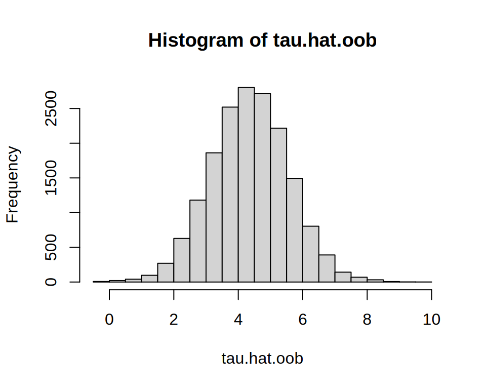
The histogram shows most students have effects near the overall ATE, with some variation. To assess whether these capture meaningful heterogeneity, we estimate the area under the TOC:
rate.oob <- rank_average_treatment_effect(c.forest, tau.hat.oob)
t.stat.oob <- rate.oob$estimate / rate.oob$std.err
pnorm(t.stat.oob, lower.tail = FALSE)  # one-sided p-value Pr(>t)
#> [1] 0.65
Here we use out-of-bag predictions both to construct \(\hat\tau(\cdot)\) and to evaluate the TOC. Since the same data are reused, exact finite-sample guarantees for the resulting \(t\)-statistic are not available. Instead of performing an explicit train/test split, we adopt a pragmatic heuristic and report a one-sided test in the direction of interest (AUTOC \(> 0\)). In this example, the one-sided test does not reject the null of no heterogeneity.
However, the TOC remains useful for evaluating alternative
prioritization strategies. For example, students with low financial
autonomy may benefit more. The causal forest variable importance
confirms financial.autonomy.index is a key predictor:
var.imp <- variable_importance(c.forest)
head(colnames(X)[order(var.imp, decreasing = TRUE)])
#> [1] "financial.autonomy.index"           "intention.to.save.index"
#> [3] "family.receives.cash.transfer"      "father.attened.secondary.school"
#> [5] "is.female"                          "has.computer.with.internet.at.home"
We can construct a TOC prioritizing students with lower financial autonomy:
rate.autonomy <- rank_average_treatment_effect(
  c.forest,
  -1 * X$financial.autonomy.index, # Negate priorities to rank by lowest first.
  q = seq(0.05, 1, length.out = 100),
  subset = !is.na(X$financial.autonomy.index))
plot(rate.autonomy, main = "TOC: By increasing financial autonomy")
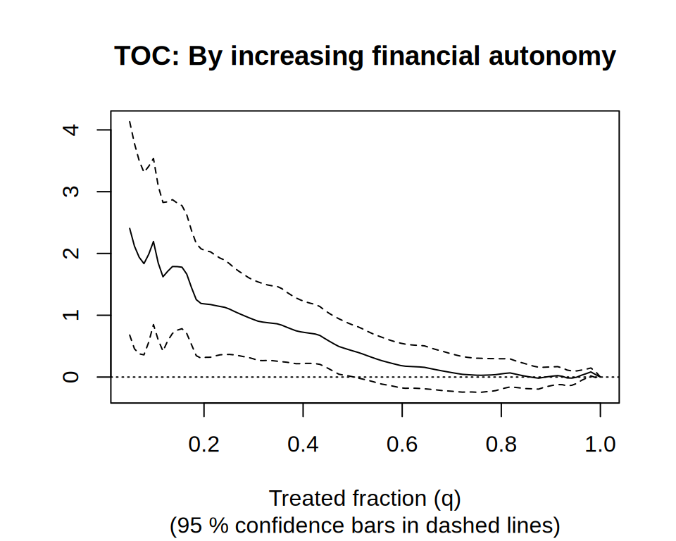
This reveals that students in the lower 20% of financial autonomy have an ATE roughly 1.1 points above the overall average, with a confidence interval excluding zero.
Training programs like these typically require resources to implement and scale to many students. The analysis here suggests that targeting students with low financial autonomy may be a desirable strategy. If we estimate the area under this TOC we get a \(t\)-value above 1.96. We would reject a null at conventional levels, leading us to conclude this prioritization strategy is effective.
rate.autonomy
#>  estimate std.err             target
#>      0.69    0.22 priorities | AUTOC
rate.autonomy$estimate / rate.autonomy$std.err
#> [1] 3.2
Next, we consider learning a simple policy that maps covariates
X to a treatment decision using the policytree
package. We perform this task on the observations without missing
covariate values. First, we retrieve doubly robust scores for the
quantities \(\text{E}[Y_i(0)]\) and
\(\text{E}[Y_i(1)]\) using the function
double_robust_scores from the policytree
package.
library(policytree)

Gamma.hat <- double_robust_scores(c.forest)
no.missing <- complete.cases(X)
X.nm <- X[no.missing, ]
Gamma.nm <- Gamma.hat[no.missing, ]
A doubly robust estimate of the average financial proficiency score in the two treatment states is
colMeans(Gamma.nm)
#> control treated
#>      58      62
In this application, it is hard to imagine that some students do not benefit from the treatment, and the treat everyone policy likely increases the overall financial proficiency of the population. Treating everyone is costly; hence, it is natural to ask if there is a policy that delivers an overall population benefit on a cost-adjusted basis. Here, we imagine we are paying the ATE when we assign treatment and offset this in our objective:
Gamma.nm[, "treated"] <- Gamma.nm[, "treated"] - ate["estimate"]
Then, we let policy_tree perform the maximization \[
\underset{\pi \in \text{depth-1 trees}}{\text{argmax}}
\frac{1}{n}\sum_{i=1}^{n} \hat \Gamma[\pi(X_i)],
\] where \(\pi(X_i) \in \{1,
2\}\) corresponds to the control and treated column of the
Gamma matrix.
ptree <- policy_tree(X.nm, Gamma.nm, depth = 1)
plot(ptree)
Here, we arrive at the simple decision rule “assign financial
education training program if financial autonomy score is \(\leq\) 41”, reaffirming our previous
analysis that indicated the pre-treatment variable
financial.autonomy.index could serve as a good candidate
for treatment decisions (Note: in practice, we would have set
aside a held-out test set to estimate the value of this policy).
Example: The effect of poverty on attention
In this section, we analyze experimental data originally studied by
Carvalho et al. (2016).
The authors conducted a randomized experiment in which low-income
individuals completed a cognitive test either before payday or after
payday. The outcome is the number of correct answers on a test designed
to measure cognitive ability. The original study did not find a
statistically significant average effect. However, subsequent analyses
suggest that poverty may impair cognitive function for certain subgroups
(Farbmacher et al., 2021). A
processed version of the data is available in grf. It
contains around 2,500 individuals and 24 pre-treatment characteristics
(age, income, education, etc.). Education is coded ordinally (4: college
graduate; 3: some college; 2: high school graduate; 1: less than high
school), and may therefore be used directly in the random forest
splitting.
We code treatment status so that \(W_i=1\) if the individual was observed after payday. With this coding, positive treatment effects correspond to improved cognitive performance (i.e., reduced impairment). This choice simplifies interpretation: for example, the TOC curve is then positive when prioritization successfully targets individuals who benefit most. Using potential outcomes notation, let \(Y_i(1)\) denote the number of correct answers under “no poverty” (after payday) and \(Y_i(0)\) the number under financial distress (before payday). The average treatment is \[ \text{E}[Y_i(1) - Y_i(0)], \] which measures the average improvement in cognitive performance when individuals are not financially constrained. The CATE then captures heterogeneity in this improvement.
data("attentionrct")
Y <- attentionrct$outcome.correct.ans.per.second
W <- 1 - attentionrct$treatment
X <- attentionrct[-(1:4)]
Given the moderate sample size relative to the number of predictors, fitting a CATE estimator on all covariates with train/test evaluation may be underpowered. To reduce dimensionality, we first estimate the conditional mean \(\text{E}[Y_i \mid X_i]\) and use forest variable importance to select a subset of covariates for the CATE. In the example below, keeping the top 10 variables by importance is a simple heuristic.
train <- sample(nrow(X), nrow(X) * 0.6)
test <- -train

Y.forest <- regression_forest(X[train, ], Y[train], num.trees = 500)
varimp.Y <- variable_importance(Y.forest)
keep <- colnames(X)[order(varimp.Y, decreasing = TRUE)[1:10]]
X.cate <- X[, keep]
print(keep)
#>  [1] "age"                               "working"
#>  [3] "education"                         "current.income"
#>  [5] "pay.day.amount.fraction.of.income" "black"
#>  [7] "household.income"                  "white"
#>  [9] "disabled"                          "retired"
Next, we fit a CATE forest on the training sample and evaluate
heterogeneity on the held-out test sample. Because the data come from a
randomized experiment, we supply the known randomization probability
through the W.hat argument.
# Estimate CATE function.
Y.hat.train <- predict(Y.forest)$predictions
cate.forest <- causal_forest(
  X.cate[train, ],
  Y[train],
  W[train],
  Y.hat = Y.hat.train,
  W.hat = 0.5
)
tau.hat.eval <- predict(cate.forest, X.cate[test, ])$predictions

# Fit evaluation forest.
eval.forest <- causal_forest(
  X[test, ],
  Y[test],
  W[test],
  W.hat = 0.5
)
Next, we assess whether the estimated CATEs captures heterogeneity in cognitive impairment by estimating the TOC and area under the TOC.
rate.cate <- rank_average_treatment_effect(
  eval.forest,
  tau.hat.eval,
  q = seq(0.05, 1, length.out = 100)
)
print(rate.cate)
#>  estimate std.err             target
#>    0.0061  0.0092 priorities | AUTOC
rate.cate$estimate / rate.cate$std.err # t-statistic
#> [1] 0.67

plot(rate.cate, main = "TOC: By decreasing CATEs")
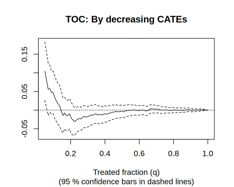
The AUTOC is not statistically distinguishable from zero at conventional levels. However, visual inspection of the TOC curve suggests that a small subset of individuals may experience an effect. If one is willing to pre-specify a quantile, this can be formally assessed by examining the confidence interval at that point on the TOC curve.
References
Athey, Susan, Julie Tibshirani, and Stefan Wager. “Generalized random forests.” The Annals of Statistics 47, no. 2 (2019): 1148-1178.
Athey, Susan, and Stefan Wager. “Estimating treatment effects with causal forests: An application.” Observational studies 5, no. 2 (2019): 37-51.
Athey, Susan, and Stefan Wager. “Policy learning with observational data.” Econometrica 89, no. 1 (2021): 133-161.
Breiman, Leo. “Random forests.” Machine learning 45, no. 1 (2001): 5-32.
Bruhn, Miriam, Luciana de Souza Leão, Arianna Legovini, Rogelio Marchetti, and Bilal Zia. “The impact of high school financial education: Evidence from a large-scale evaluation in Brazil.” American Economic Journal: Applied Economics 8, no. 4 (2016).
Carvalho, Leandro S., Stephan Meier, and Stephanie W. Wang. “Poverty and economic decision-making: Evidence from changes in financial resources at payday.” American Economic Review 106, no. 2 (2016): 260-84.
Chernozhukov, Victor, Denis Chetverikov, Mert Demirer, Esther Duflo, Christian Hansen, Whitney Newey, and James Robins. “Double/debiased machine learning for treatment and structural parameters.” The Econometrics Journal, 2018.
Cui, Yifan, Michael R. Kosorok, Erik Sverdrup, Stefan Wager, and Ruoqing Zhu. “Estimating heterogeneous treatment effects with right-censored data via causal survival forests.” Journal of the Royal Statistical Society Series B: Statistical Methodology 85, no. 2 (2023): 179-211.
Dandl, Susanne, Christian Haslinger, Torsten Hothorn, Heidi Seibold, Erik Sverdrup, Stefan Wager, and Achim Zeileis. “What makes forest-based heterogeneous treatment effect estimators work?.” The Annals of Applied Statistics 18, no. 1 (2024): 506-528.
Efron, Bradley. “Prediction, estimation, and attribution.” International Statistical Review 88 (2020): S28-S59.
Farbmacher, Helmut, Heinrich Kögel, and Martin Spindler. “Heterogeneous effects of poverty on attention.” Labour Economics 71 (2021): 102028.
Friedberg, Rina, Julie Tibshirani, Susan Athey, and Stefan Wager. “Local linear forests.” Journal of Computational and Graphical Statistics 30, no. 2 (2020): 503-517.
James, Gareth, Daniela Witten, Trevor Hastie, and Robert Tibshirani. An introduction to statistical learning: with applications in R. Vol. 103. New York: springer, 2013.
Mayer, Imke, Erik Sverdrup, Tobias Gauss, Jean-Denis Moyer, Stefan Wager, and Julie Josse. “Doubly robust treatment effect estimation with missing attributes.” The Annals of Applied Statistics 14, no. 3 (2020): 1409-1431.
Robins, James M., Andrea Rotnitzky, and Lue Ping Zhao. “Estimation of regression coefficients when some regressors are not always observed.” Journal of the American Statistical Association 89, no. 427 (1994): 846-866.
Nie, Xinkun, and Stefan Wager. “Quasi-oracle estimation of heterogeneous treatment effects.” Biometrika 108, no. 2 (2021): 299-319.
Robinson, Peter M. “Root-N-consistent semiparametric regression.” Econometrica: Journal of the Econometric Society (1988): 931-954.
Rosenbaum, Paul R., and Donald B. Rubin. “The central role of the propensity score in observational studies for causal effects.” Biometrika 70, no. 1 (1983): 41-55.
Sverdrup, Erik, Maria Petukhova, and Stefan Wager. “Estimating treatment effect heterogeneity in psychiatry: A review and tutorial with causal forests.” International Journal of Methods in Psychiatric Research 34, no. 2 (2025): e70015.
Sverdrup, Erik, Han Wu, Susan Athey, and Stefan Wager. “Qini curves for multi-armed treatment rules.” Journal of Computational and Graphical Statistics 34, no. 3 (2025): 948-960.
Sverdrup, Erik, Ayush Kanodia, Zhengyuan Zhou, Susan Athey, and Stefan Wager. “policytree: Policy learning via doubly robust empirical welfare maximization over trees.” Journal of Open Source Software 5, no. 50 (2020): 2232.
Twala, Bheki ETH, M. C. Jones, and David J. Hand. “Good methods for coping with missing data in decision trees.” Pattern Recognition Letters 29, no. 7 (2008): 950-956.
Zheng, Wenjing, and Mark J. van der Laan. “Cross-validated targeted minimum-loss-based estimation.” In Targeted Learning, pp. 459-474. Springer, New York, NY, 2011.
Wager, Stefan. Causal Inference: A Statistical Learning Approach. Cambridge University Press (in preparation), 2024.
Wager, Stefan. Sequential validation of treatment heterogeneity. arXiv preprint arXiv:2405.05534 (2024).
Wager, Stefan, and Susan Athey. “Estimation and inference of heterogeneous treatment effects using random forests.” Journal of the American Statistical Association 113.523 (2018): 1228-1242.
Yadlowsky, Steve, Scott Fleming, Nigam Shah, Emma Brunskill, and Stefan Wager. “Evaluating Treatment Prioritization Rules via Rank-Weighted Average Treatment Effects.” Journal of the American Statistical Association, 120(549), 2025.
Zeileis, Achim, Torsten Hothorn, and Kurt Hornik. “Model-based recursive partitioning.” Journal of Computational and Graphical Statistics 17, no. 2 (2008): 492-514.