Predict with a lm forest — predict.lm

Gets estimates of $h_k(x)$, k = 1..K in the conditionally linear model $Y = c(x) + h_1(x)W_1 + ... + h_K(x)W_K$, for a target sample X = x.

# S3 method for lm_forest
predict(
  object,
  newdata = NULL,
  num.threads = NULL,
  estimate.variance = FALSE,
  drop = FALSE,
  ...
)

Arguments

object	The trained forest.
newdata	Points at which predictions should be made. If NULL, makes out-of-bag predictions on the training set instead (i.e., provides predictions at Xi using only trees that did not use the i-th training example). Note that this matrix should have the number of columns as the training matrix, and that the columns must appear in the same order.
num.threads	Number of threads used in training. If set to NULL, the software automatically selects an appropriate amount.
estimate.variance	Whether variance estimates for $\hat h_k(x)$ are desired (for confidence intervals). This option is currently only supported for univariate outcomes Y.
drop	If TRUE, coerce the prediction result to the lowest possible dimension. Default is FALSE.
...	Additional arguments (currently ignored).

Value

A list with elements `predictions`: a 3d array of dimension [num.samples, K, M] with predictions for regressor W, for each outcome 1,..,M (singleton dimensions in this array can be dropped by passing the `drop` argument to `[`, or with the shorthand `$predictions[,,]`), and optionally `variance.estimates`: a matrix with K columns with variance estimates.

Examples

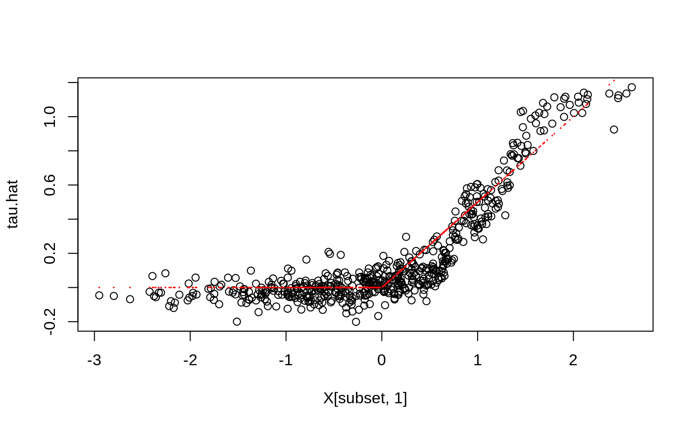
# \donttest{
if (require("rdd", quietly = TRUE)) {
# Train a LM Forest to estimate CATEs in a regression discontinuity design.
# Simulate a simple example with a heterogeneous jump in the CEF.
n <- 2000
p <- 5
X <- matrix(rnorm(n * p), n, p)
Z <- runif(n, -4, 4)
cutoff <- 0
W <- as.numeric(Z >= cutoff)
tau <- pmax(0.5 * X[, 1], 0)
Y <- tau * W  + 1 / (1 + exp(2 * Z)) + 0.2 * rnorm(n)

# Compute the Imbens-Kalyanaraman MSE-optimal bandwidth for a local linear regression.
bandwidth <- IKbandwidth(Z, Y, cutoff)
# Compute kernel weights for a triangular kernel.
sample.weights <- kernelwts(Z, cutoff, bandwidth, "triangular")

# Alternatively, specify bandwith and triangular kernel weights without using the `rdd` package.
# bandwidth <- # user can hand-specify this.
# dist <- abs((Z - cutoff) / bandwidth)
# sample.weights <- (1 - dist) * (dist <= 1) / bandwidth

# Estimate a local linear regression with the running variable Z conditional on covariates X = x:
# Y = c(x) + tau(x) W + b(x) Z.
# Specify gradient.weights = c(1, 0) to target heterogeneity in the RDD coefficient tau(x).
# Also, fit forest on subset with non-zero weights for faster estimation.
subset <- sample.weights > 0
lmf <- lm_forest(X[subset, ], Y[subset], cbind(W, Z)[subset, ],
                 sample.weights = sample.weights[subset], gradient.weights = c(1, 0))
tau.hat <- predict(lmf)$predictions[, 1, ]

# Plot estimated tau(x) vs simulated ground truth.
plot(X[subset, 1], tau.hat)
points(X[subset, 1], tau[subset], col = "red", cex = 0.1)
}
# }