Predict with a multi arm causal forest — predict.multi_arm_causal

Gets estimates of contrasts tau_k(x) using a trained multi arm causal forest (k = 1,...,K-1 where K is the number of treatments).

# S3 method for multi_arm_causal_forest
predict(
  object,
  newdata = NULL,
  num.threads = NULL,
  estimate.variance = FALSE,
  drop = FALSE,
  ...
)

Arguments

object	The trained forest.
newdata	Points at which predictions should be made. If NULL, makes out-of-bag predictions on the training set instead (i.e., provides predictions at Xi using only trees that did not use the i-th training example). Note that this matrix should have the number of columns as the training matrix, and that the columns must appear in the same order.
num.threads	Number of threads used in training. If set to NULL, the software automatically selects an appropriate amount.
estimate.variance	Whether variance estimates for $\hat\tau(x)$ are desired (for confidence intervals). This option is currently only supported for univariate outcomes Y.
drop	If TRUE, coerce the prediction result to the lowest possible dimension. Default is FALSE.
...	Additional arguments (currently ignored).

Value

A list with elements `predictions`: a 3d array of dimension [num.samples, K-1, M] with predictions for each contrast, for each outcome 1,..,M (singleton dimensions in this array can be dropped by passing the `drop` argument to `[`, or with the shorthand `$predictions[,,]`), and optionally `variance.estimates`: a matrix with K-1 columns with variance estimates for each contrast.

Examples

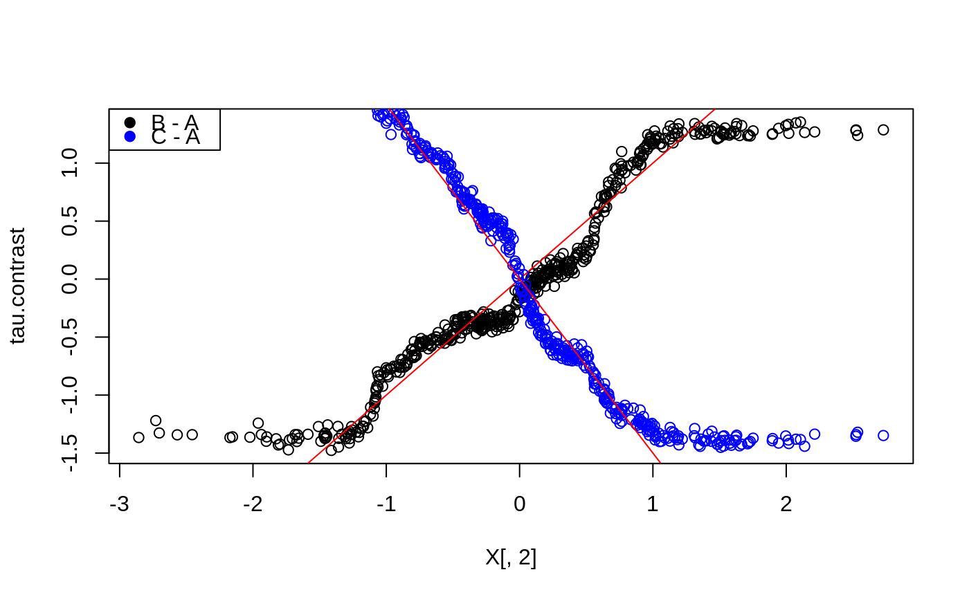
# \donttest{
# Train a multi arm causal forest.
n <- 500
p <- 10
X <- matrix(rnorm(n * p), n, p)
W <- as.factor(sample(c("A", "B", "C"), n, replace = TRUE))
Y <- X[, 1] + X[, 2] * (W == "B") - 1.5 * X[, 2] * (W == "C") + rnorm(n)
mc.forest <- multi_arm_causal_forest(X, Y, W)

# Predict contrasts (out-of-bag) using the forest.
# Fitting several outcomes jointly is supported, and the returned prediction array has
# dimension [num.samples, num.contrasts, num.outcomes]. Since num.outcomes is one in
# this example, we use drop = TRUE to ignore this singleton dimension.
mc.pred <- predict(mc.forest, drop = TRUE)

# By default, the first ordinal treatment is used as baseline ("A" in this example),
# giving two contrasts tau_B = Y(B) - Y(A), tau_C = Y(C) - Y(A)
tau.hat <- mc.pred$predictions

plot(X[, 2], tau.hat[, "B - A"], ylab = "tau.contrast")
abline(0, 1, col = "red")
points(X[, 2], tau.hat[, "C - A"], col = "blue")
abline(0, -1.5, col = "red")
legend("topleft", c("B - A", "C - A"), col = c("black", "blue"), pch = 19)

# The average treatment effect of the arms with "A" as baseline.
average_treatment_effect(mc.forest)
#>          estimate   std.err contrast outcome
#> B - A -0.07847752 0.1243464    B - A     Y.1
#> C - A  0.05486383 0.1344698    C - A     Y.1

# The conditional response surfaces mu_k(X) for a single outcome can be reconstructed from
# the contrasts tau_k(x), the treatment propensities e_k(x), and the conditional mean m(x).
# Given treatment "A" as baseline we have:
# m(x) := E[Y | X] = E[Y(A) | X] + E[W_B (Y(B) - Y(A))] + E[W_C (Y(C) - Y(A))]
# which given unconfoundedness is equal to:
# m(x) = mu(A, x) + e_B(x) tau_B(X) + e_C(x) tau_C(x)
# Rearranging and plugging in the above expressions, we obtain the following estimates
# * mu(A, x) = m(x) - e_B(x) tau_B(x) - e_C(x) tau_C(x)
# * mu(B, x) = m(x) + (1 - e_B(x)) tau_B(x) - e_C(x) tau_C(x)
# * mu(C, x) = m(x) - e_B(x) tau_B(x) + (1 - e_C(x)) tau_C(x)
Y.hat <- mc.forest$Y.hat
W.hat <- mc.forest$W.hat

muA <- Y.hat - W.hat[, "B"] * tau.hat[, "B - A"] - W.hat[, "C"] * tau.hat[, "C - A"]
muB <- Y.hat + (1 - W.hat[, "B"]) * tau.hat[, "B - A"] - W.hat[, "C"] * tau.hat[, "C - A"]
muC <- Y.hat - W.hat[, "B"] * tau.hat[, "B - A"] + (1 - W.hat[, "C"]) * tau.hat[, "C - A"]

# These can also be obtained with some array manipulations.
# (the first column is always the baseline arm)
Y.hat.baseline <- Y.hat - rowSums(W.hat[, -1, drop = FALSE] * tau.hat)
mu.hat.matrix <- cbind(Y.hat.baseline, c(Y.hat.baseline) + tau.hat)
colnames(mu.hat.matrix) <- levels(W)
head(mu.hat.matrix)
#>               A          B          C
#> [1,] -1.0185650 -0.9957107 -1.6314533
#> [2,] -1.5850962 -2.1119223 -0.5363287
#> [3,]  1.2633944  2.2884232  0.0451462
#> [4,]  0.9006375  0.3766952  1.9331346
#> [5,] -1.2029916 -1.0871341 -1.8426707
#> [6,]  1.4559153  1.3479929  1.5000191

# The reference level for contrast prediction can be changed with `relevel`.
# Fit and predict with treatment B as baseline:
W <- relevel(W, ref = "B")
mc.forest.B <- multi_arm_causal_forest(X, Y, W)
# }